basic-use
basic-use.RmdCitation
Please cite as
Dan MacLean. (2019). TeamMacLean/besthr: Initial Release (0.3.0). Zenodo. https://doi.org/10.5281/zenodo.3374507
Simplest Use Case - Two Groups, No Replicates
With a data frame or similar object, use the estimate()
function to get the bootstrap estimates of the ranked data.
estimate() has a basic function call as follows:
estimate(data, score_column_name, group_column_name, control = control_group_name)
The first argument after the
library(besthr)
hr_data_1_file <- system.file("extdata", "example-data-1.csv", package = "besthr")
hr_data_1 <- readr::read_csv(hr_data_1_file)
#> Rows: 20 Columns: 2
#> ── Column specification ────────────────────────────────────────────────────────
#> Delimiter: ","
#> chr (1): group
#> dbl (1): score
#>
#> ℹ Use `spec()` to retrieve the full column specification for this data.
#> ℹ Specify the column types or set `show_col_types = FALSE` to quiet this message.
head(hr_data_1)
#> # A tibble: 6 × 2
#> score group
#> <dbl> <chr>
#> 1 10 A
#> 2 9 A
#> 3 10 A
#> 4 10 A
#> 5 8 A
#> 6 8 A
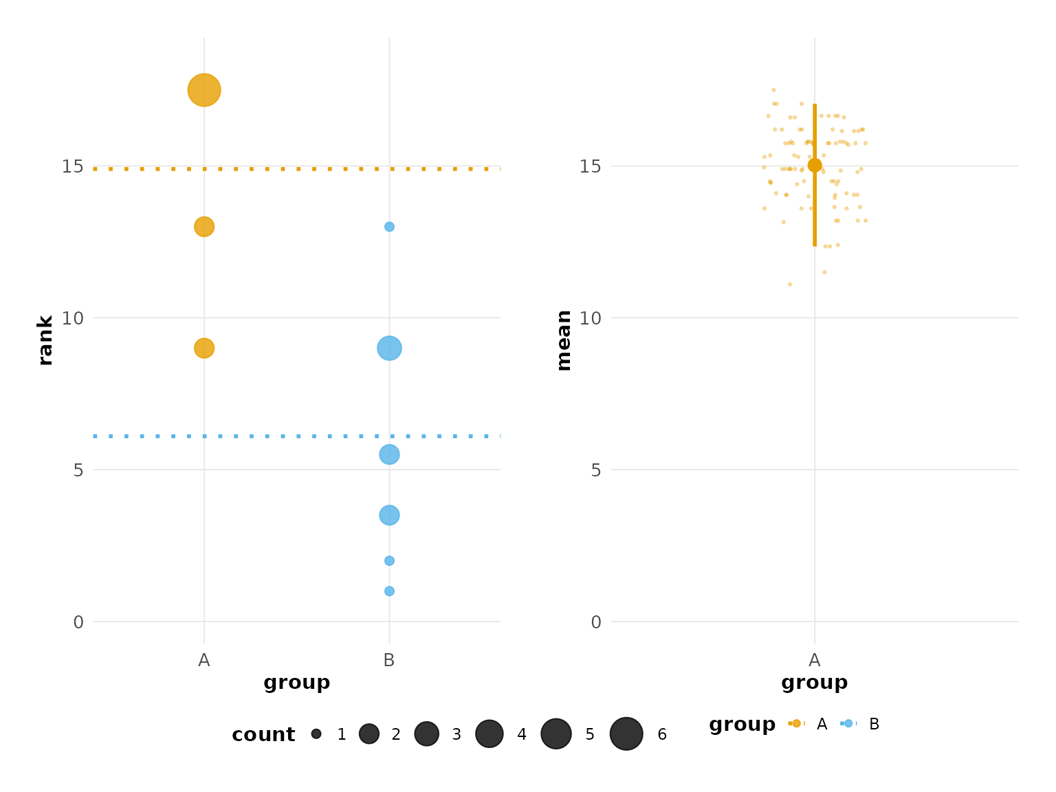
hr_est_1 <- estimate(hr_data_1, score, group, control = "A")
hr_est_1
#> besthr (HR Rank Score Analysis with Bootstrap Estimation)
#> =========================================================
#>
#> Control: A
#>
#> Unpaired mean rank difference of A (14.9, n=10) minus B (6.1, n=10)
#> 8.8
#> Confidence Intervals (0.025, 0.975)
#> 4.02125, 8.9525
#>
#> 100 bootstrap resamples.
plot(hr_est_1)
#> Confidence interval: 2.5% - 97.5%
Setting Options
You may select the group to set as the common reference control with
control.
You may select the number of iterations of the bootstrap to perform
with nits and the quantiles for the confidence interval
with low and high.
estimate(hr_data_1, score, group, control = "A", nits = 1000, low = 0.4, high = 0.6) %>%
  plot()
#> Confidence interval: 40.0% - 60.0%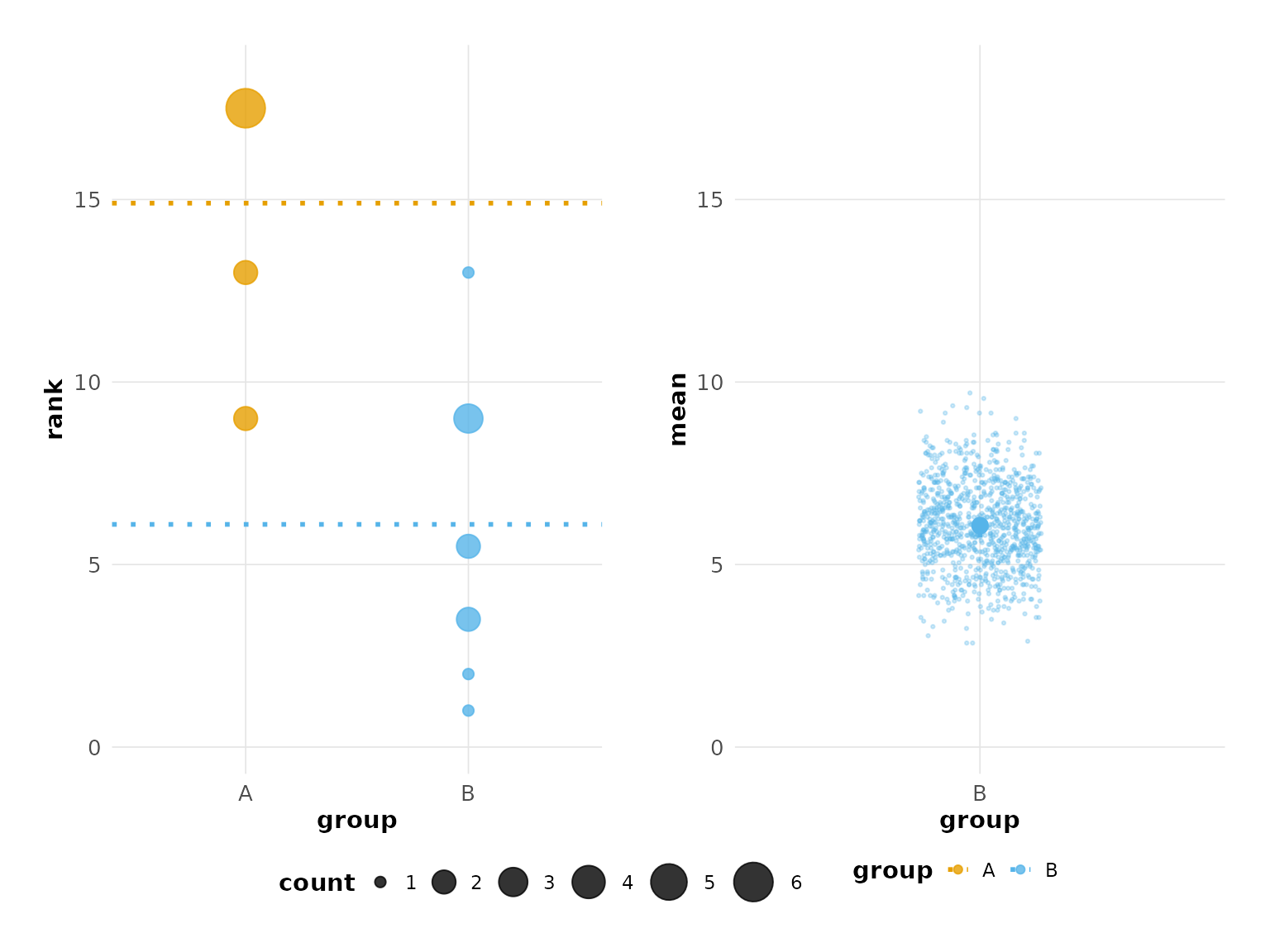
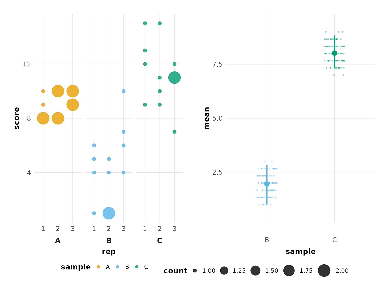
Extended Use Case - Technical Replicates
You can extend the estimate() options to specify a third
column in the data that contains technical replicate information, add
the technical replicate column name after the sample column. Technical
replicates are automatically merged using the mean()
function before ranking.
hr_data_3_file <- system.file("extdata", "example-data-3.csv", package = "besthr")
hr_data_3 <- readr::read_csv(hr_data_3_file)
#> Rows: 36 Columns: 3
#> ── Column specification ────────────────────────────────────────────────────────
#> Delimiter: ","
#> chr (1): sample
#> dbl (2): score, rep
#>
#> ℹ Use `spec()` to retrieve the full column specification for this data.
#> ℹ Specify the column types or set `show_col_types = FALSE` to quiet this message.
head(hr_data_3)
#> # A tibble: 6 × 3
#>   score sample   rep
#>   <dbl> <chr>  <dbl>
#> 1     8 A          1
#> 2     9 A          1
#> 3     8 A          1
#> 4    10 A          1
#> 5     8 A          2
#> 6     8 A          2

hr_est_3 <- estimate(hr_data_3, score, sample, rep, control = "A")

hr_est_3
#> besthr (HR Rank Score Analysis with Bootstrap Estimation)
#> =========================================================
#>
#> Control: A
#>
#> Unpaired mean rank difference of A (5, n=3) minus B (2, n=3)
#>  3
#> Confidence Intervals (0.025, 0.975)
#>  1, 2.84166666666666
#>
#> Unpaired mean rank difference of A (5, n=3) minus C (8, n=3)
#>  -3
#> Confidence Intervals (0.025, 0.975)
#>  7.33333333333333, 8.84166666666666
#>
#> 100 bootstrap resamples.

plot(hr_est_3)
#> Confidence interval: 2.5% - 97.5%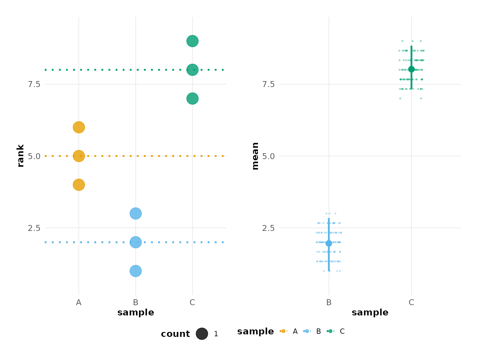
Built-in Themes and Color Palettes
besthr uses a modern, colorblind-safe appearance by default. You can customize the look using themes and color palettes.
Theme Options
Use the theme parameter to change the overall visual
style:
-
"modern"(default) - A clean, contemporary style with refined typography -
"classic"- The original besthr appearance (for backward compatibility)
# Modern theme (default)
plot(hr_est_1)
#> Confidence interval: 2.5% - 97.5%
# Classic theme (original style)
plot(hr_est_1, theme = "classic")
#> Confidence interval: 2.5% - 97.5%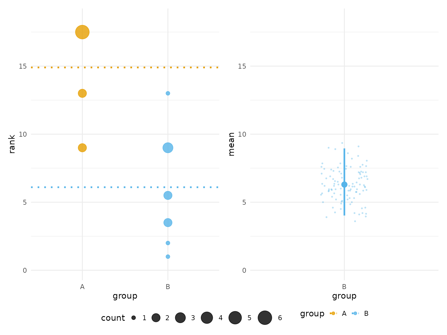
Color Palette Options
Use the colors parameter to change the color
palette:
-
"okabe_ito"(default) - Colorblind-safe Okabe-Ito palette -
"default"- Original besthr colors (for backward compatibility) -
"viridis"- Viridis color scale
# Default is already colorblind-safe
plot(hr_est_1)
#> Confidence interval: 2.5% - 97.5%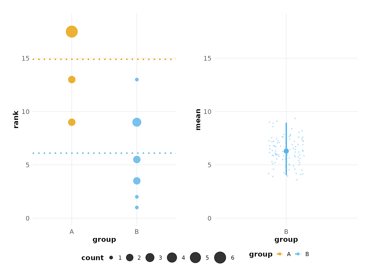
# Original colors
plot(hr_est_1, colors = "default")
#> Confidence interval: 2.5% - 97.5%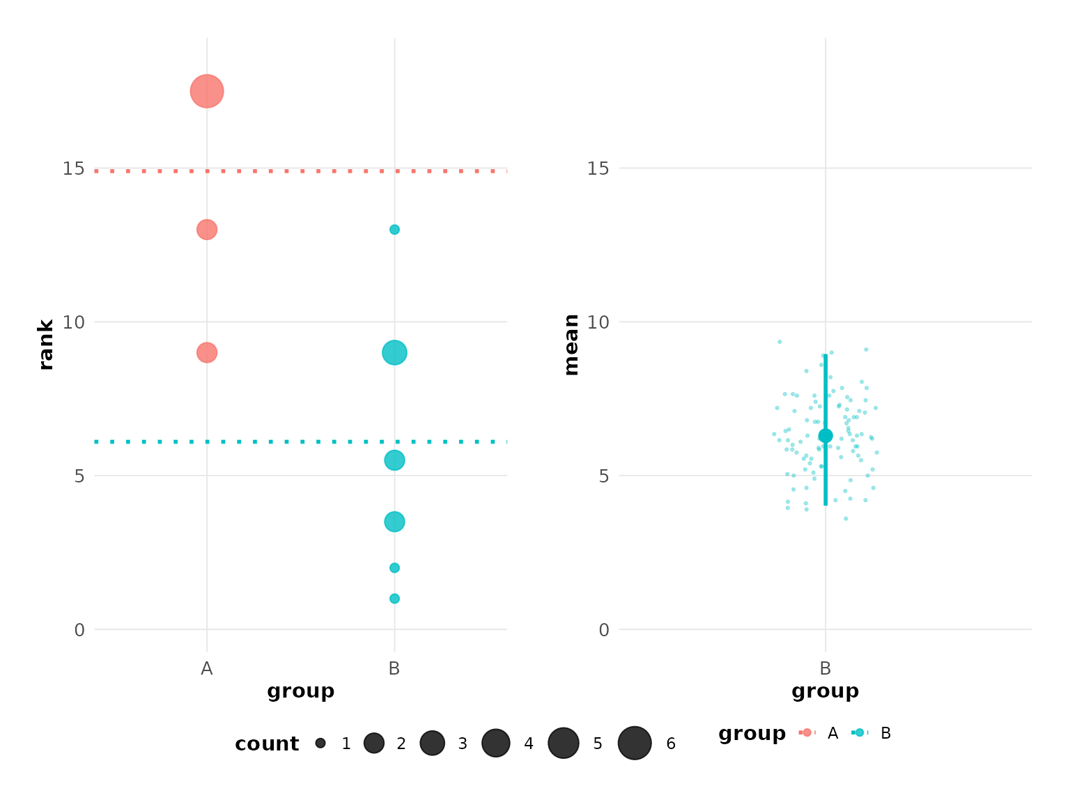
# Viridis palette
plot(hr_est_1, colors = "viridis")
#> Confidence interval: 2.5% - 97.5%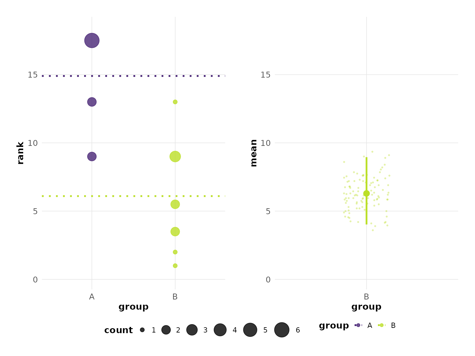
Quick Style Presets
For easy customization without understanding all options, use preset styles:
# Publication-ready style
plot(hr_est_1, config = besthr_style("publication"))
#> Confidence interval: 2.5% - 97.5%
# Presentation style (larger elements)
plot(hr_est_1, config = besthr_style("presentation"))
#> Confidence interval: 2.5% - 97.5%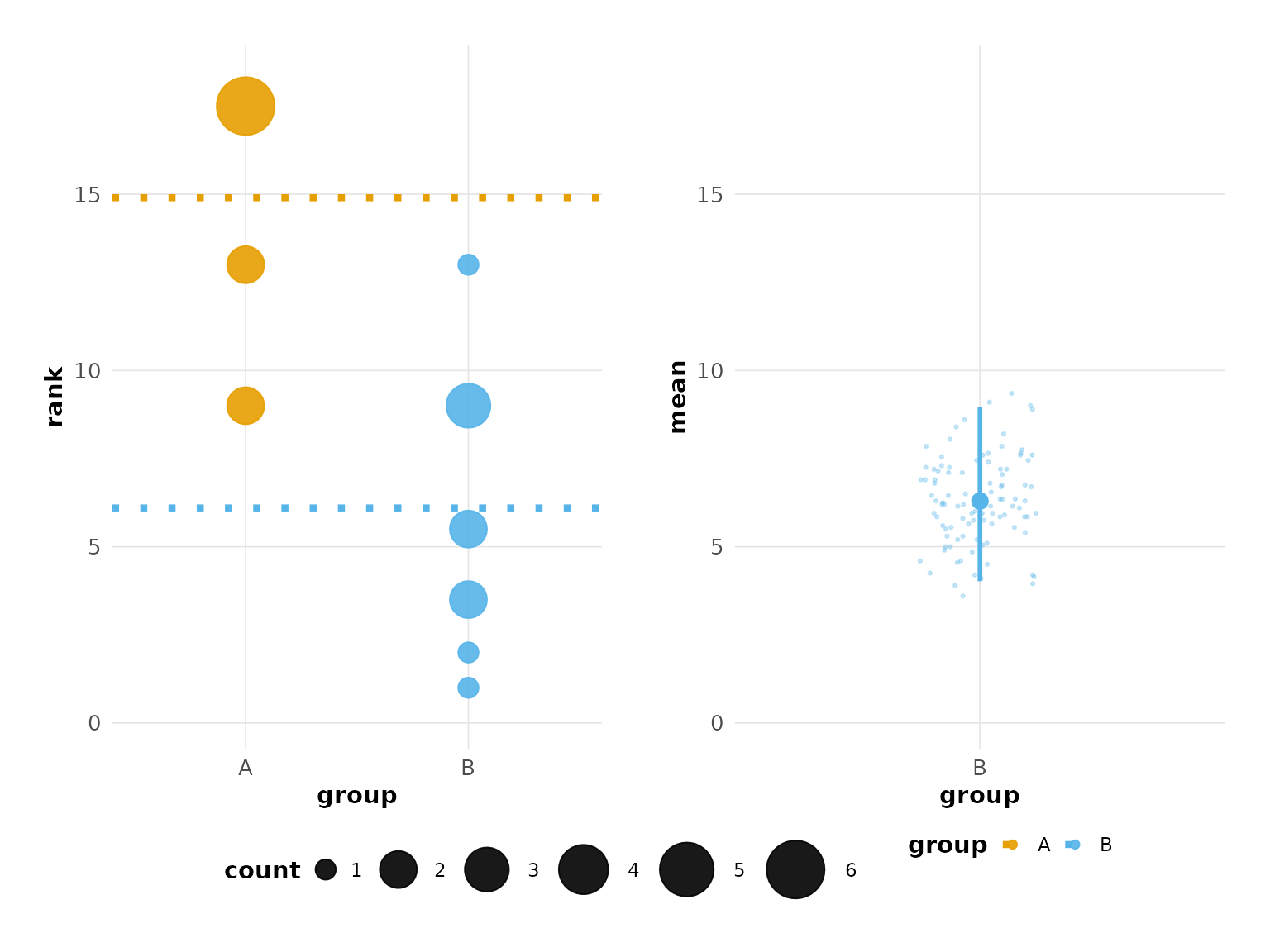
# Density style (gradient density instead of points)
plot(hr_est_1, config = besthr_style("density"))
#> Confidence interval: 2.5% - 97.5%
#> Picking joint bandwidth of 0.441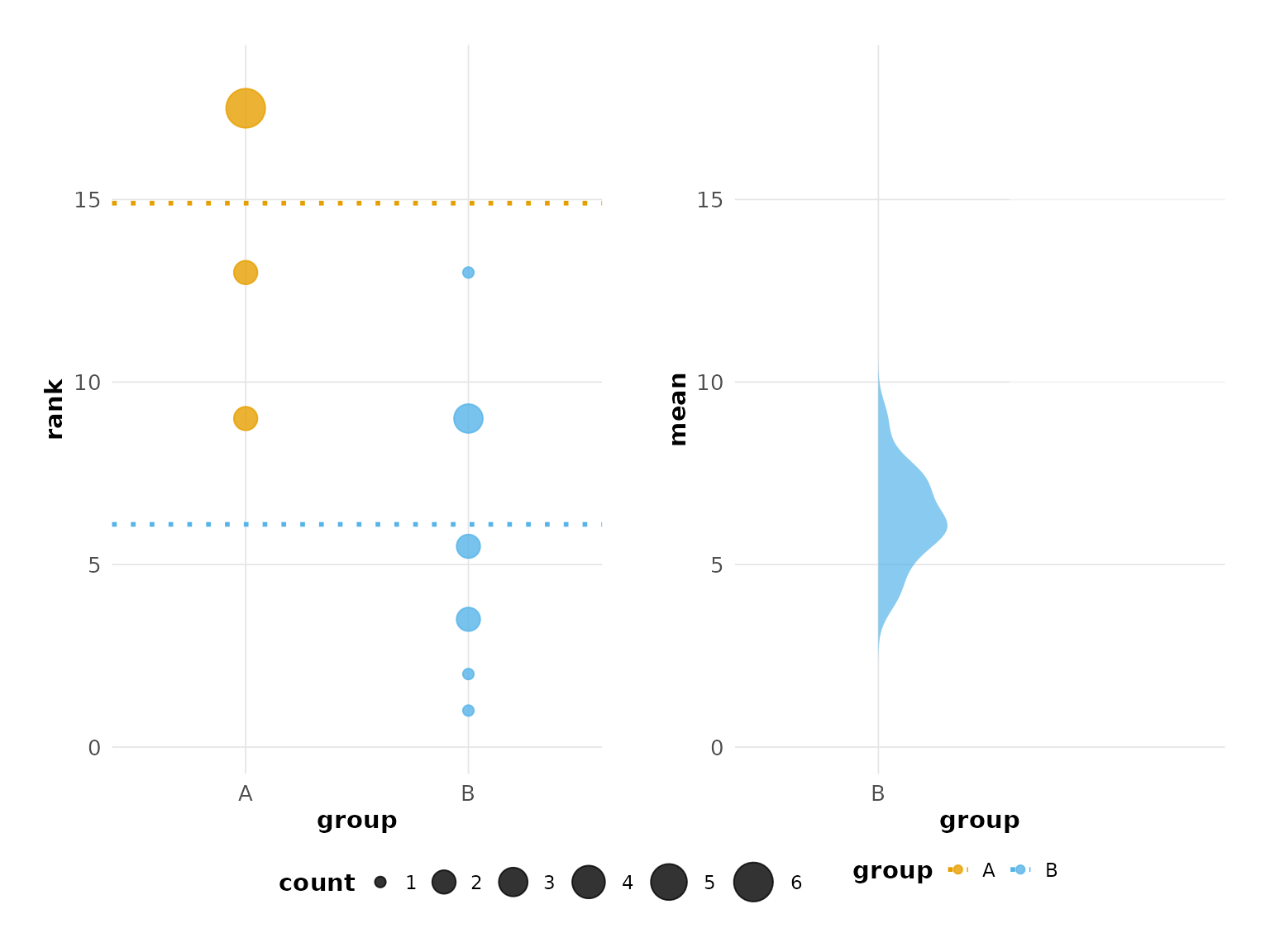
# See all available styles
list_besthr_styles()
#> Available besthr style presets:
#>
#>   'default'       Modern theme with colorblind-safe colors (recommended)
#>   'classic'       Original besthr appearance
#>   'publication'   Clean style for journal figures
#>   'presentation'  Larger elements for slides
#>   'density'       Gradient density display for bootstrap
#>
#> Usage: plot(hr, config = besthr_style('publication'))
Using besthr Palettes Directly
The color palettes can also be used directly in your own ggplot2 code:
# Get palette colors
besthr_palette("okabe_ito", n = 4)
#> [1] "#E69F00" "#56B4E9" "#009E73" "#F0E442"

# Available palettes
besthr_palette("default", n = 3)
#> [1] "#F8766D" "#00BA38" "#619CFF"
besthr_palette("viridis", n = 3)
#> [1] "#482576FF" "#21908CFF" "#BBDF27FF"
Styling Plots
Using Built-in Themes and Colors
The easiest way to style your plots is using the theme
and colors parameters:
# Modern look with colorblind-safe colors (this is the default)
plot(hr_est_1, theme = "modern", colors = "okabe_ito")
#> Confidence interval: 2.5% - 97.5%
# Classic appearance (original besthr style)
plot(hr_est_1, theme = "classic", colors = "default")
#> Confidence interval: 2.5% - 97.5%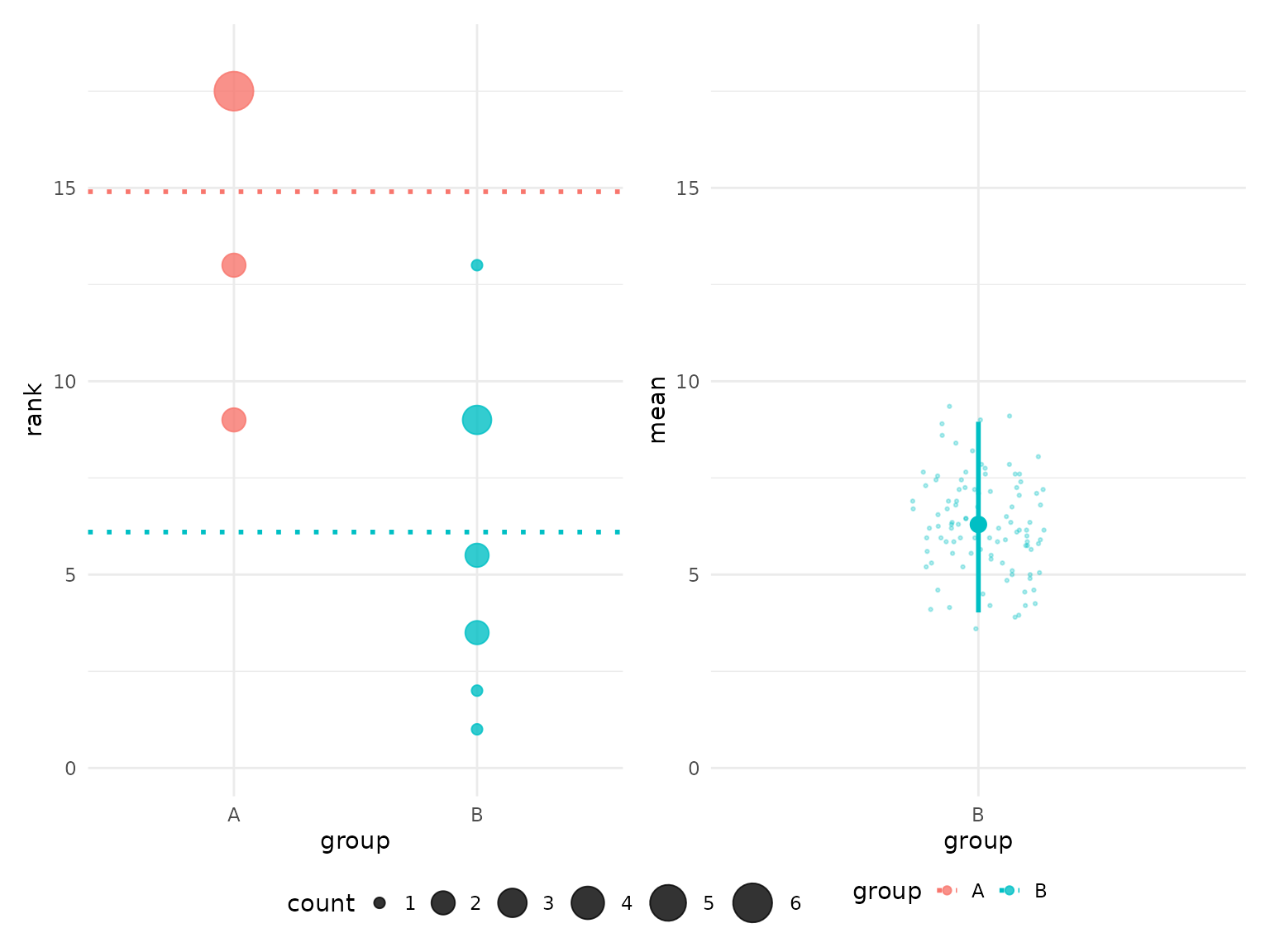
# Viridis color scheme
plot(hr_est_1, colors = "viridis")
#> Confidence interval: 2.5% - 97.5%
Adding Titles and Annotations
The plot object is a patchwork composition. You can add
titles using plot_annotation():
library(patchwork)

p <- plot(hr_est_1)
#> Confidence interval: 2.5% - 97.5%

p + plot_annotation(
  title = 'HR Score Analysis',
  subtitle = "Control vs Treatment",
  caption = 'Generated with besthr'
)
Advanced Configuration
For users who need fine-grained control over plot appearance, besthr provides a configuration system.
Using besthr_plot_config
The besthr_plot_config() function creates a
configuration object that controls all aspects of plot appearance:
# Create a custom configuration
cfg <- besthr_plot_config(
  panel_widths = c(2, 1),        # Make data panel wider than bootstrap panel
  point_size_range = c(3, 10),   # Larger points
  point_alpha = 0.9,             # More opaque points
  mean_line_width = 1.5,         # Thicker mean lines
  theme_style = "modern",
  color_palette = "okabe_ito"
)

print(cfg)
#> besthr plot configuration:
#>   Panel widths: 2, 1
#>   Y-axis limits: auto
#>   Y-axis expand: 0.05
#>   Point size range: 3 - 10
#>   Point alpha: 0.9
#>   Mean line type: 3
#>   Mean line width: 1.5
#>   Density alpha: 0.7
#>   Density style: points
#>   Theme: modern
#>   Colors: okabe_ito
# Use the configuration in plot
plot(hr_est_1, config = cfg)
#> Confidence interval: 2.5% - 97.5%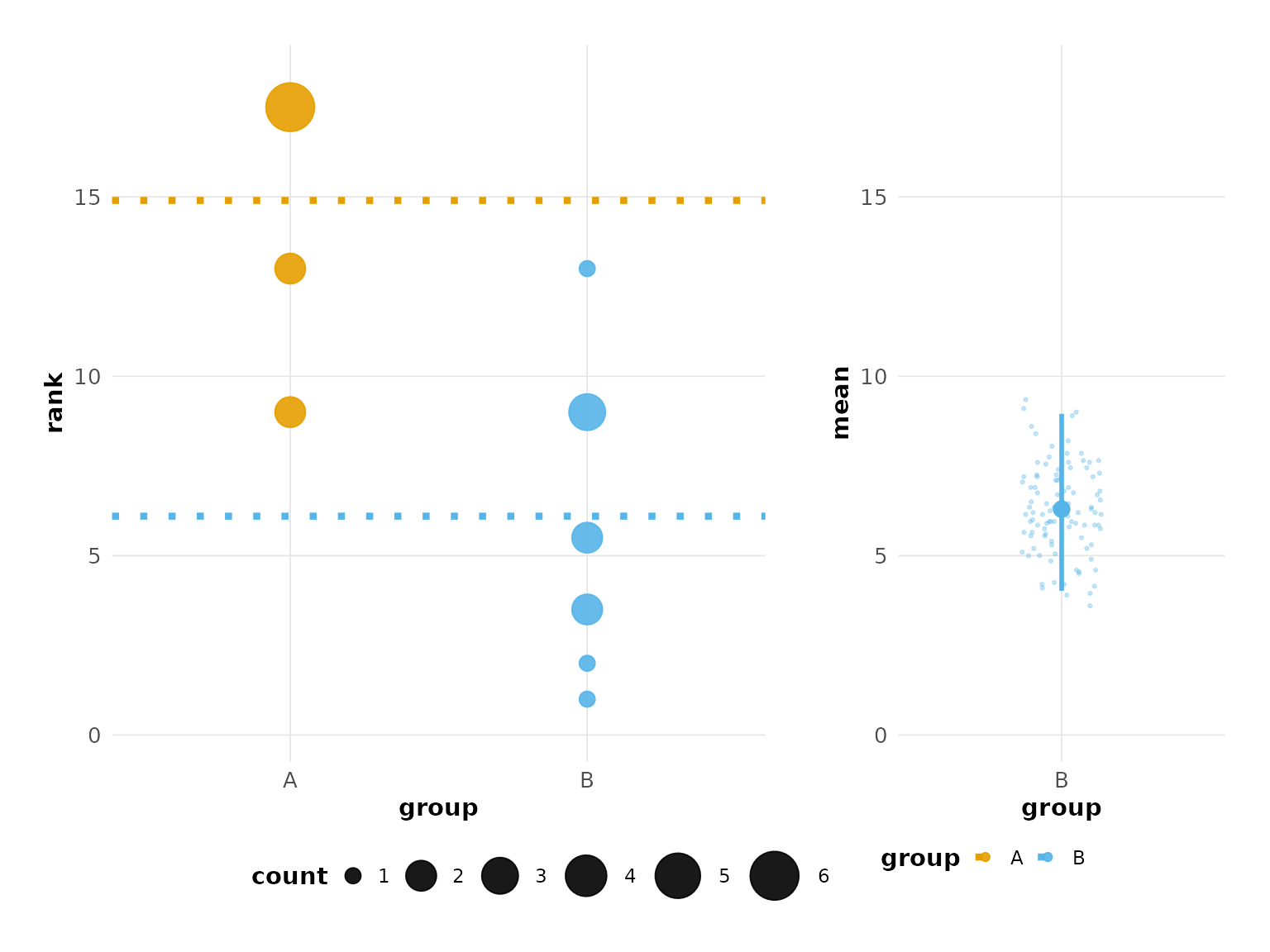
You can update an existing configuration with
update_config():
# Modify just one setting
cfg2 <- update_config(cfg, panel_widths = c(1, 2))
plot(hr_est_1, config = cfg2)
#> Confidence interval: 2.5% - 97.5%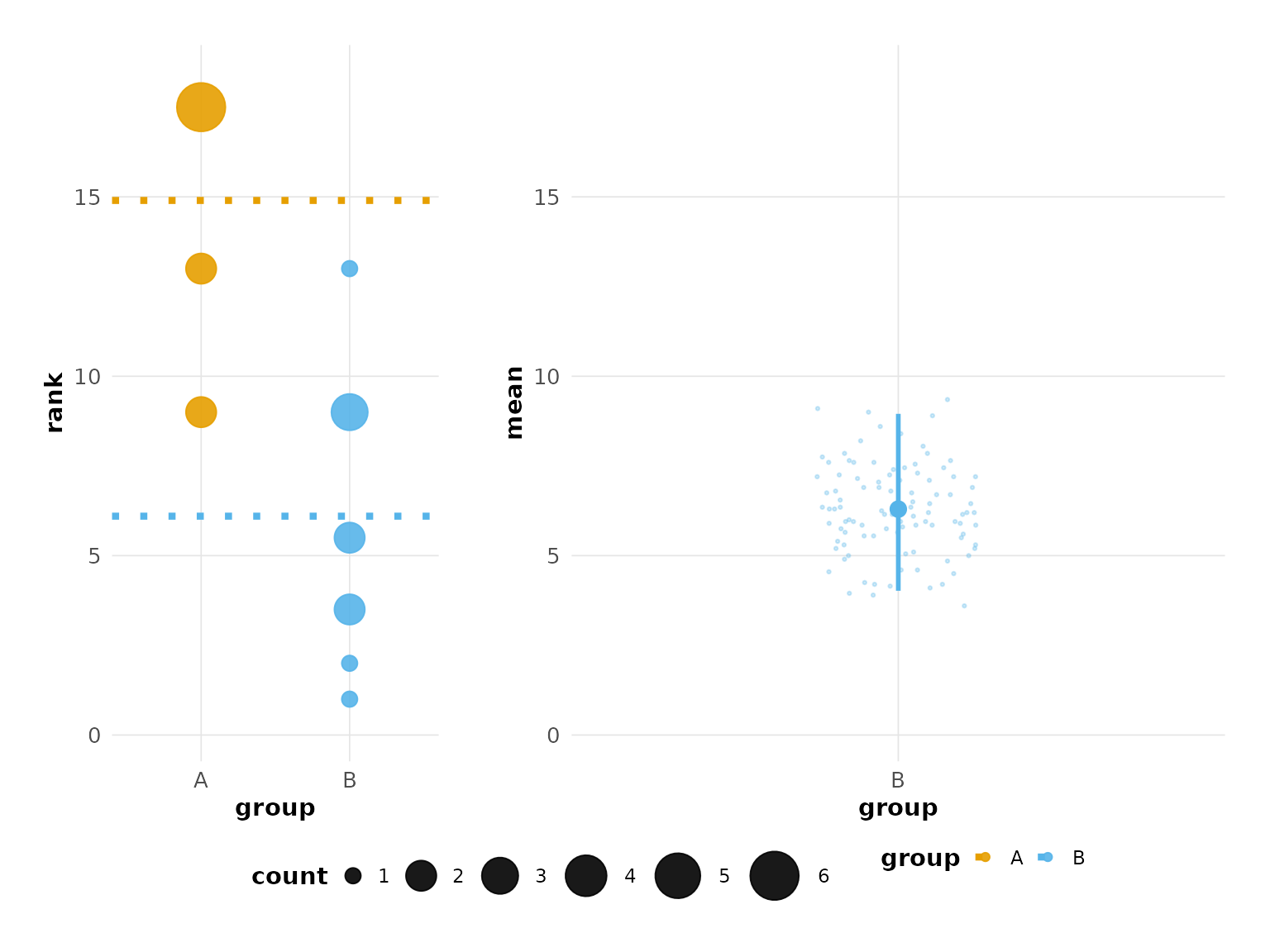
Configuration Options
| Parameter | Default | Description |
|---|---|---|
panel_widths |
c(1, 1) |
Relative widths of observation and bootstrap panels |
y_limits |
NULL (auto) |
Fixed y-axis limits, or NULL for automatic |
y_expand |
0.05 |
Proportional expansion of y-axis limits |
point_size_range |
c(2, 8) |
Min/max point sizes based on count |
point_alpha |
0.8 |
Point transparency (0-1) |
mean_line_type |
3 |
Line type for mean indicators |
mean_line_width |
1 |
Line width for mean indicators |
density_alpha |
0.7 |
Bootstrap density transparency |
density_style |
"points" |
Density display: “points” (jittered bootstrap), “gradient”, or “solid” |
theme_style |
"modern" |
Theme: “classic” or “modern” |
color_palette |
"okabe_ito" |
Colors: “default”, “okabe_ito”, or “viridis” |
Building Custom Plots
For maximum flexibility, you can build plots from individual components.
Using besthr_data_view
The besthr_data_view() function extracts all plotting
data from an hrest object with unified axis limits:
# Create a data view
dv <- besthr_data_view(hr_est_1)
print(dv)
#> besthr data view:
#>   Groups: 2
#>   Observations: 20
#>   Bootstrap iterations: 100
#>   Rank limits: 0.17 - 18.32
#>   Control: A

# Access the data
head(dv$ranked)
#> # A tibble: 6 × 3
#>   score group  rank
#>   <dbl> <chr> <dbl>
#> 1    10 A      17.5
#> 2     9 A      13
#> 3    10 A      17.5
#> 4    10 A      17.5
#> 5     8 A       9
#> 6     8 A       9
head(dv$bootstrap)
#> # A tibble: 6 × 3
#>   group  mean iteration
#>   <chr> <dbl>     <int>
#> 1 B      5.95         1
#> 2 B      5.85         2
#> 3 B      6.35         3
#> 4 B      5            4
#> 5 B      5.8          5
#> 6 B      5.9          6
dv$rank_limits
#> [1]  0.175 18.325
Using Panel Builders
You can build individual panels and compose them yourself:
library(patchwork)

# Create panels
cfg <- besthr_plot_config(theme_style = "modern", color_palette = "okabe_ito")
dv <- besthr_data_view(hr_est_1, cfg)

p1 <- build_observation_panel(dv, cfg, "rank_simulation")
p2 <- build_bootstrap_panel(dv, cfg)

# Custom composition with different widths
p1 + p2 + plot_layout(widths = c(3, 1))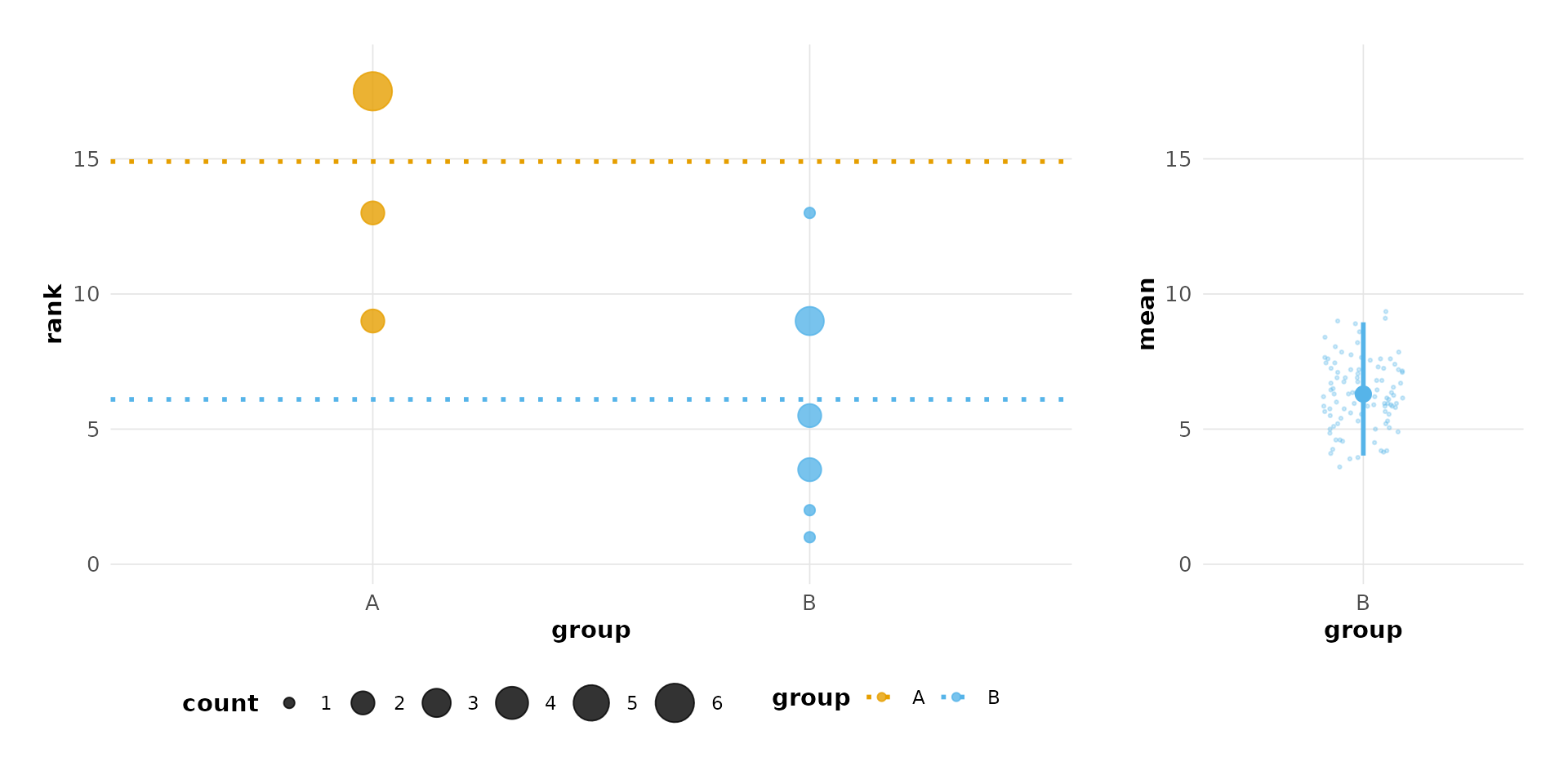
Alternative Visualizations
Raincloud Plots
The plot_raincloud() function provides an alternative
visualization showing jittered data points with confidence
intervals:
plot_raincloud(hr_est_1)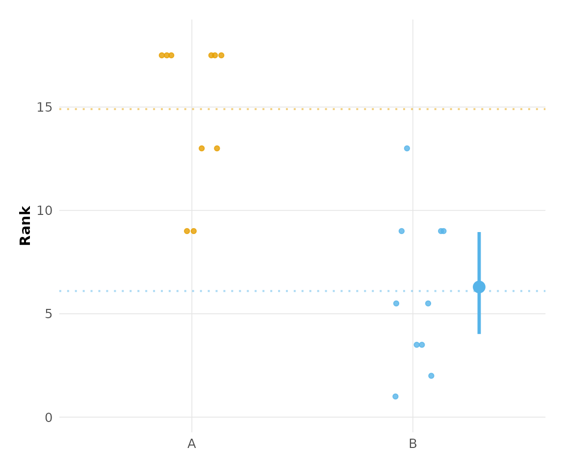
# With modern styling
plot_raincloud(hr_est_1, theme = "modern", colors = "okabe_ito")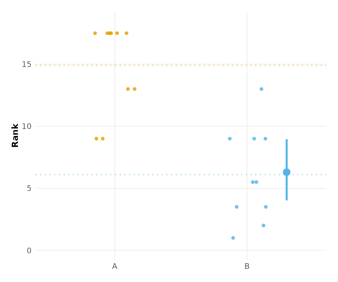
Bootstrap Raincloud
The plot_bootstrap_raincloud() function shows the
bootstrap distribution as jittered points:
plot_bootstrap_raincloud(hr_est_1)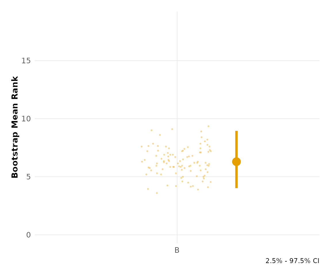
CI Color Customization
The derive_ci_colors() function generates confidence
interval colors that harmonize with the selected palette:
# Default CI colors
derive_ci_colors("default", "classic")
#> [1] "#0000FFA0" "#A0A0A0A0" "#FF0000A0"

# Okabe-Ito derived CI colors
derive_ci_colors("okabe_ito", "modern")
#> [1] "#0072B2AA" "#999999AA" "#D55E00AA"

# Viridis derived CI colors
derive_ci_colors("viridis", "classic")
#> [1] "#440154AB" "#21908CAB" "#FDE725AB"
Significance and Effect Size
# Create example data with 3 groups and realistic variation
set.seed(42)
d_effect <- data.frame(
  score = c(
    sample(1:4, 12, replace = TRUE),   # Group A: low scores (control)
    sample(4:8, 12, replace = TRUE),   # Group B: medium-high scores
    sample(6:10, 12, replace = TRUE)   # Group C: high scores
  ),
  group = rep(c("A", "B", "C"), each = 12)
)
hr_effect <- estimate(d_effect, score, group, control = "A", nits = 1000)
Significance Annotations
Add significance stars to groups where the bootstrap confidence interval does not overlap the control mean:
plot(hr_effect, show_significance = TRUE)
#> Confidence interval: 2.5% - 97.5%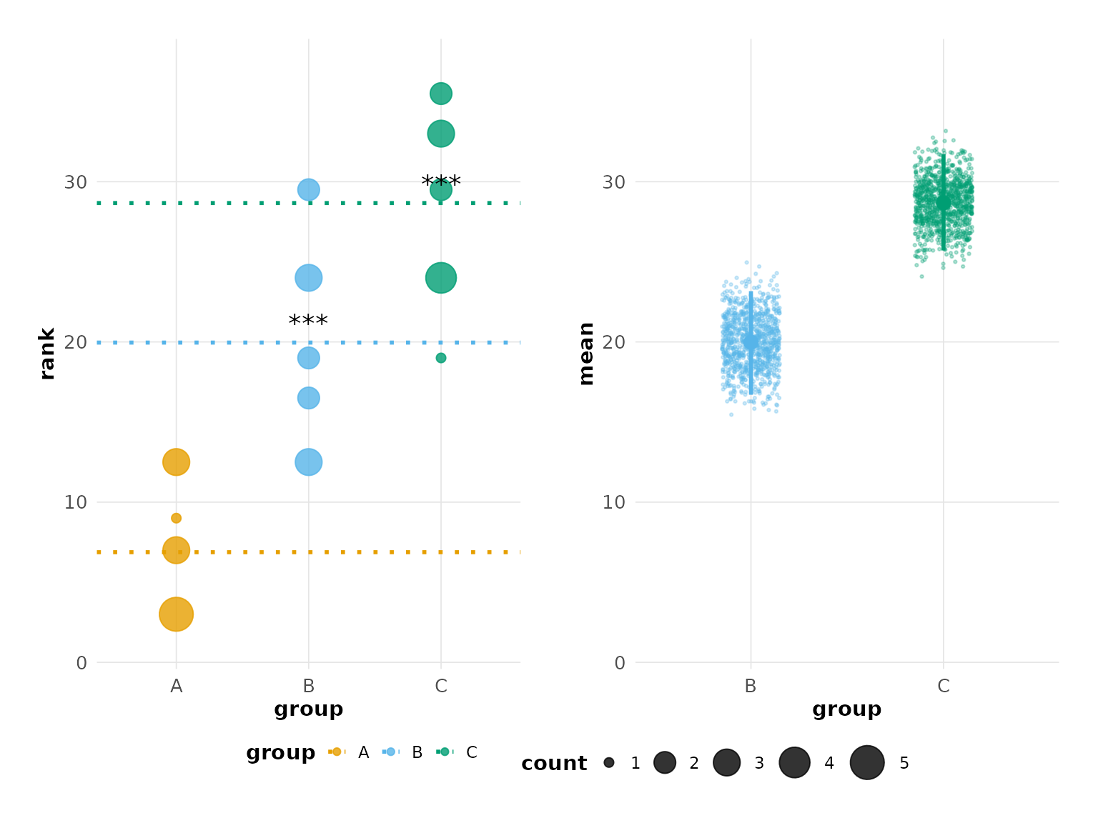
Effect Size Annotation
Display effect size (difference from control) with confidence intervals:
plot(hr_effect, show_effect_size = TRUE)
#> Confidence interval: 2.5% - 97.5%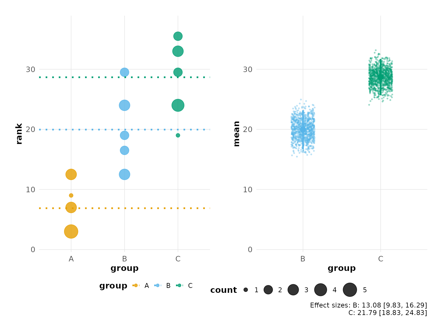
Computing Statistics Directly
You can access the significance and effect size calculations directly:
# Compute significance
compute_significance(hr_effect)
#>   group significant p_value stars
#> 1     A          NA      NA
#> 2     B        TRUE       0   ***
#> 3     C        TRUE       0   ***

# Compute effect sizes
compute_effect_size(hr_effect)
#>   group   effect effect_ci_low effect_ci_high
#> 1     A       NA            NA             NA
#> 2     B 13.08333      9.830208       16.29271
#> 3     C 21.79167     18.833333       24.83333
Summary Tables
Generate publication-ready summary tables with
besthr_table():
# Default tibble format
besthr_table(hr_effect)
#> # A tibble: 3 × 6
#>   group     n mean_rank ci_low ci_high effect_size
#>   <chr> <int>     <dbl>  <dbl>   <dbl>       <dbl>
#> 1 A        12      6.88   NA      NA          NA
#> 2 B        12     20.0    16.7    23.2        13.1
#> 3 C        12     28.7    25.7    31.7        21.8

# With significance stars
besthr_table(hr_effect, include_significance = TRUE)
#> # A tibble: 3 × 7
#>   group     n mean_rank ci_low ci_high effect_size significance
#>   <chr> <int>     <dbl>  <dbl>   <dbl>       <dbl> <chr>
#> 1 A        12      6.88   NA      NA          NA   ""
#> 2 B        12     20.0    16.7    23.2        13.1 "***"
#> 3 C        12     28.7    25.7    31.7        21.8 "***"

# Markdown format
besthr_table(hr_est_1, format = "markdown")
#> [1] "| group | n | mean_rank | ci_low | ci_high | effect_size |\n| --- | --- | --- | --- | --- | --- |\n| A | 10 | 14.9 | NA | NA | NA |\n| B | 10 |  6.1 | 4.02 | 8.95 | -8.8 |"
Other formats available: "html",
"latex"
Publication Export
Save plots directly to publication-quality files:
# Save to PNG (default 300 DPI)
save_besthr(hr_est_1, "figure1.png")

# Save to PDF
save_besthr(hr_est_1, "figure1.pdf", width = 10, height = 8)

# Save raincloud plot
save_besthr(hr_est_1, "raincloud.png", type = "raincloud")

# With custom options
save_besthr(hr_est_1, "figure1.png",
            theme = "modern",
            colors = "okabe_ito",
            width = 10,
            height = 6,
            dpi = 600)
Supported formats: PNG, PDF, SVG, TIFF, JPEG