Dan MacLean 18 March, 2026
Synopsis
besthr is a package that creates plots showing scored HR experiments and plots of distribution of means of ranks of HR score from bootstrapping.
Installation
You can install from CRAN in the usual way.
install.packages("besthr")

# or for the dev version
#install.packages("devtools")
devtools::install_github("TeamMacLean/besthr")
Citation
Please cite as
Dan MacLean. (2019). TeamMacLean/besthr: Initial Release (0.3.0). Zenodo. https://doi.org/10.5281/zenodo.3374507
Documentation
Full API docs are available here https://teammaclean.github.io/besthr/
Simplest Use Case - Two Groups, No Replicates
With a data frame or similar object, use the estimate() function to get the bootstrap estimates of the ranked data.
estimate() has a basic function call as follows:
estimate(data, score_column_name, group_column_name, control = control_group_name)
The first argument after the
library(besthr)

hr_data_1_file <- system.file("extdata", "example-data-1.csv", package = "besthr")
hr_data_1 <- readr::read_csv(hr_data_1_file)
## Rows: 20 Columns: 2
## ── Column specification ────────────────────────────────────────────────────────
## Delimiter: ","
## chr (1): group
## dbl (1): score
##
## ℹ Use `spec()` to retrieve the full column specification for this data.
## ℹ Specify the column types or set `show_col_types = FALSE` to quiet this message.
head(hr_data_1)## # A tibble: 6 × 2
## score group
## <dbl> <chr>
## 1 10 A
## 2 9 A
## 3 10 A
## 4 10 A
## 5 8 A
## 6 8 A
hr_est_1 <- estimate(hr_data_1, score, group, control = "A")
hr_est_1
## besthr (HR Rank Score Analysis with Bootstrap Estimation)
## =========================================================
##
## Control: A
##
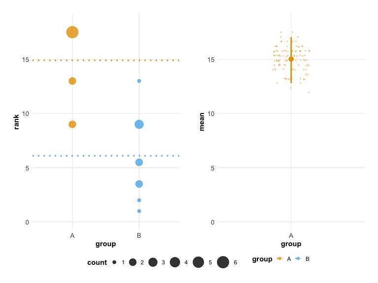
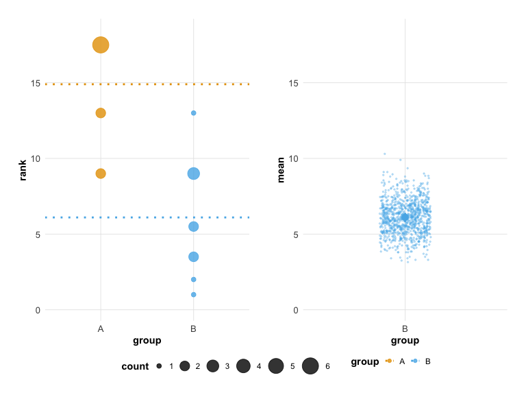
## Unpaired mean rank difference of A (14.9, n=10) minus B (6.1, n=10)
## 8.8
## Confidence Intervals (0.025, 0.975)
## 3.96875, 8.42875
##
## 100 bootstrap resamples.
plot(hr_est_1)
Extended Use Case - Technical Replicates
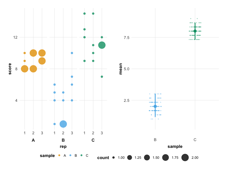
You can extend the estimate() options to specify a third column in the data that contains technical replicate information, add the technical replicate column name after the sample column. Technical replicates are automatically merged using the mean() function before ranking.
hr_data_3_file <- system.file("extdata", "example-data-3.csv", package = "besthr")
hr_data_3 <- readr::read_csv(hr_data_3_file)
## Rows: 36 Columns: 3
## ── Column specification ────────────────────────────────────────────────────────
## Delimiter: ","
## chr (1): sample
## dbl (2): score, rep
##
## ℹ Use `spec()` to retrieve the full column specification for this data.
## ℹ Specify the column types or set `show_col_types = FALSE` to quiet this message.
head(hr_data_3)## # A tibble: 6 × 3
## score sample rep
## <dbl> <chr> <dbl>
## 1 8 A 1
## 2 9 A 1
## 3 8 A 1
## 4 10 A 1
## 5 8 A 2
## 6 8 A 2
hr_est_3 <- estimate(hr_data_3, score, sample, rep, control = "A")

hr_est_3
## besthr (HR Rank Score Analysis with Bootstrap Estimation)
## =========================================================
##
## Control: A
##
## Unpaired mean rank difference of A (5, n=3) minus B (2, n=3)
## 3
## Confidence Intervals (0.025, 0.975)
## 1.15833333333333, 3
##
## Unpaired mean rank difference of A (5, n=3) minus C (8, n=3)
## -3
## Confidence Intervals (0.025, 0.975)
## 7.33333333333333, 8.66666666666667
##
## 100 bootstrap resamples.
plot(hr_est_3)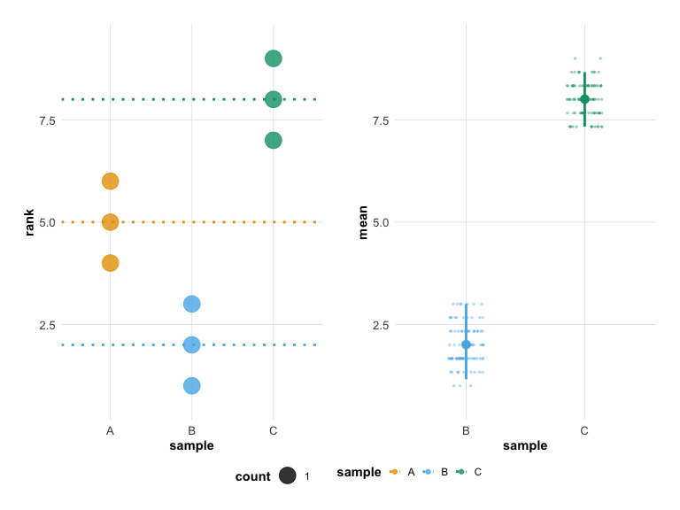
Built-in Themes and Color Palettes
besthr includes built-in themes and colorblind-safe color palettes that can be applied directly through the plot() function.
Theme Options
Use the theme parameter to change the overall visual style:
-
"classic"(default) - The original besthr appearance -
"modern"- A cleaner, contemporary style with refined typography and grid
# Classic theme (default - same as before)
plot(hr_est_1, theme = "classic")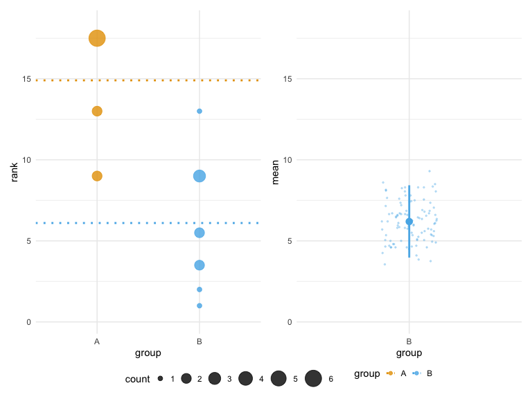
# Modern theme
plot(hr_est_1, theme = "modern")
Color Palette Options
Use the colors parameter to change the color palette:
-
"default"- Original besthr colors -
"okabe_ito"- Colorblind-safe Okabe-Ito palette -
"viridis"- Viridis color scale
# Colorblind-safe palette
plot(hr_est_1, colors = "okabe_ito")
# Viridis palette
plot(hr_est_1, colors = "viridis")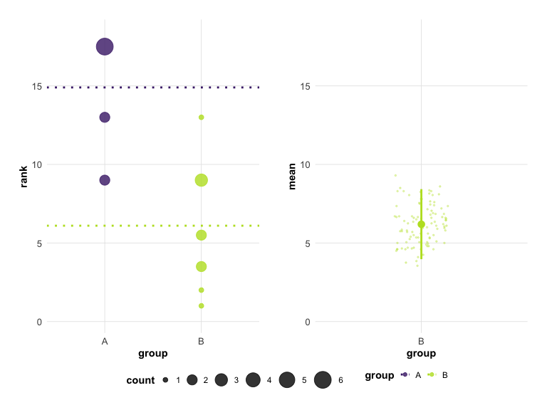
Combining Theme and Colors
You can combine both options for a fully customized look:
# Modern theme with colorblind-safe colors
plot(hr_est_1, theme = "modern", colors = "okabe_ito")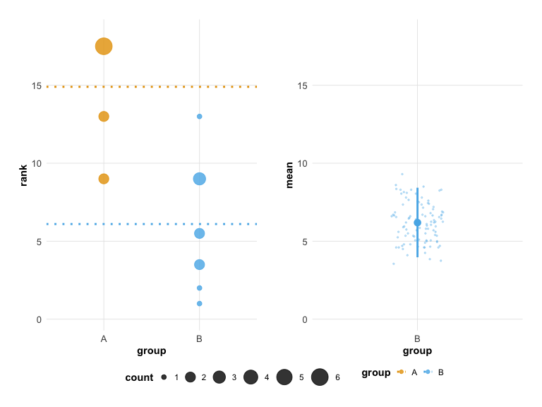
Using besthr Palettes Directly
The color palettes can also be used directly in your own ggplot2 code:
# Get palette colors
besthr_palette("okabe_ito", n = 4)
# Available palettes
besthr_palette("default", n = 3)
besthr_palette("viridis", n = 3)Styling Plots
Recommended: Use Built-in Themes and Colors
The easiest way to style your plots is using the theme and colors parameters:
# Modern look with colorblind-safe colors (this is the default)
plot(hr_est_1, theme = "modern", colors = "okabe_ito")
# Classic appearance
plot(hr_est_1, theme = "classic", colors = "default")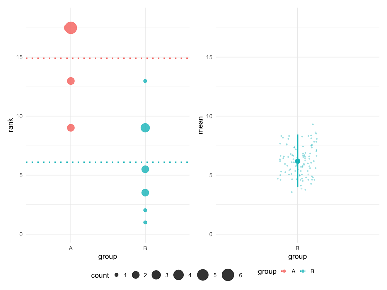
# Viridis color scheme
plot(hr_est_1, colors = "viridis")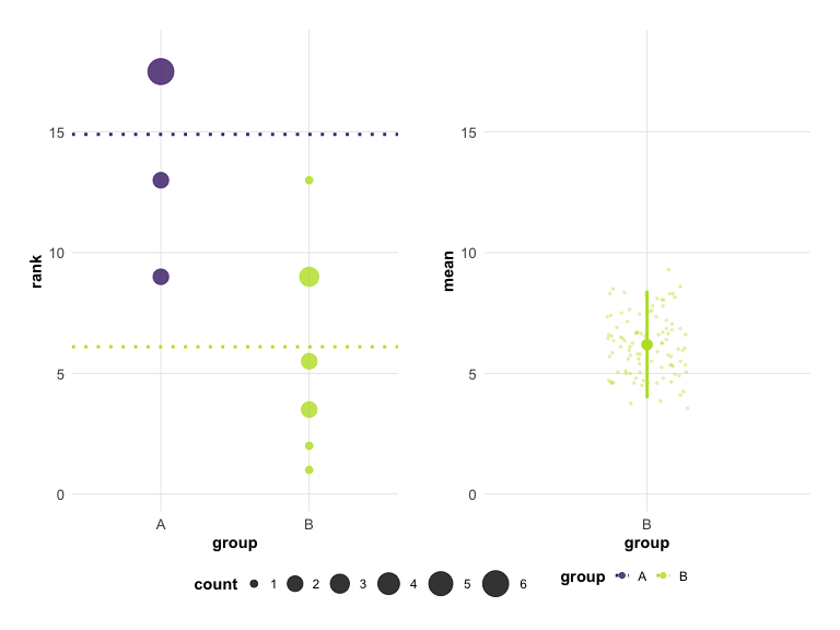
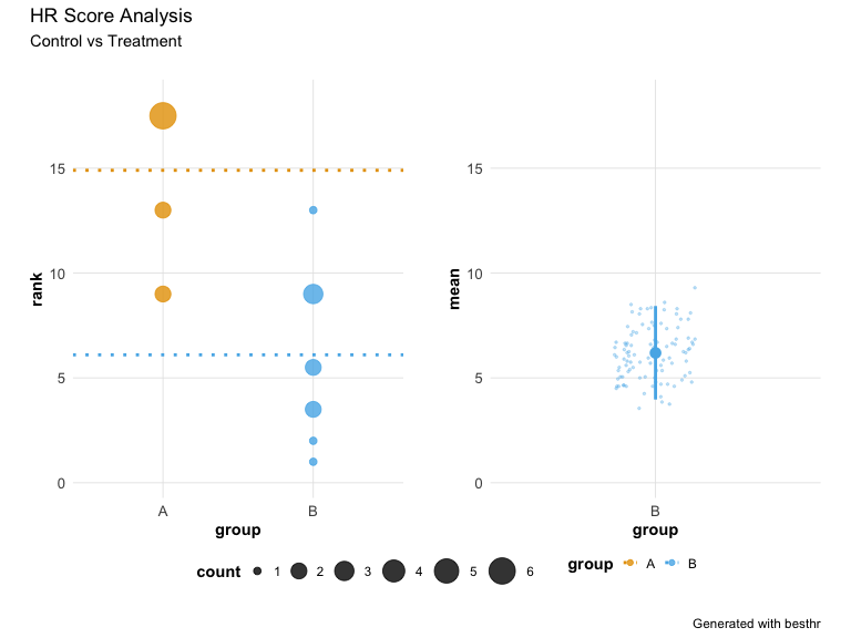
Adding Titles and Annotations
The plot object is a patchwork composition. You can add titles using plot_annotation():
p + plot_annotation(
  title = 'HR Score Analysis',
  subtitle = "Control vs Treatment",
  caption = 'Generated with besthr'
)
Raincloud Plot
For a combined view of raw data points with summary statistics, use plot_raincloud():
plot_raincloud(hr_est_1)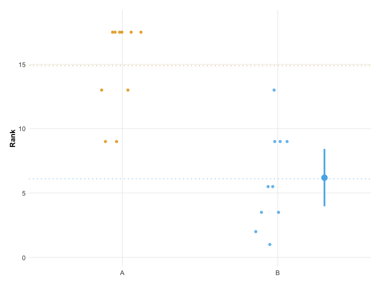
Significance and Effect Size Annotations
You can add statistical annotations to your plots to highlight significant results.
# Create example data with 3 groups and realistic variation
set.seed(42)
d_effect <- data.frame(
  score = c(
    sample(1:4, 12, replace = TRUE),   # Group A: low scores (control)
    sample(4:8, 12, replace = TRUE),   # Group B: medium-high scores
    sample(6:10, 12, replace = TRUE)   # Group C: high scores
  ),
  group = rep(c("A", "B", "C"), each = 12)
)
hr_effect <- estimate(d_effect, score, group, control = "A", nits = 1000)
Significance Stars
Add significance stars to groups where the bootstrap confidence interval does not overlap the control mean:
plot(hr_effect, show_significance = TRUE)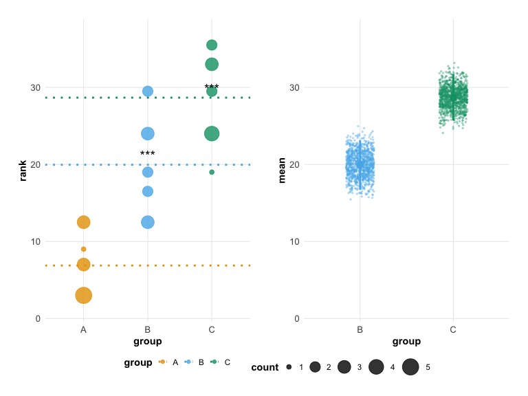
Effect Size Annotation
Display effect size (difference from control) with confidence intervals:
plot(hr_effect, show_effect_size = TRUE)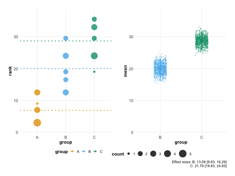
Computing Statistics Directly
You can also access the significance and effect size calculations directly:
# Compute significance
compute_significance(hr_est_1)
# Compute effect sizes
compute_effect_size(hr_est_1)Summary Tables
Generate publication-ready summary tables with besthr_table():
# Default tibble format
besthr_table(hr_effect)
## # A tibble: 3 × 6
## group n mean_rank ci_low ci_high effect_size
## <chr> <int> <dbl> <dbl> <dbl> <dbl>
## 1 A 12 6.88 NA NA NA
## 2 B 12 20.0 16.7 23.2 13.1
## 3 C 12 28.7 25.7 31.7 21.8
# With significance stars
besthr_table(hr_effect, include_significance = TRUE)
## # A tibble: 3 × 7
## group n mean_rank ci_low ci_high effect_size significance
## <chr> <int> <dbl> <dbl> <dbl> <dbl> <chr>
## 1 A 12 6.88 NA NA NA ""
## 2 B 12 20.0 16.7 23.2 13.1 "***"
## 3 C 12 28.7 25.7 31.7 21.8 "***"Export Formats
Generate tables in various formats for publication:
# Markdown format
besthr_table(hr_est_1, format = "markdown")
## [1] "| group | n | mean_rank | ci_low | ci_high | effect_size |\n| --- | --- | --- | --- | --- | --- |\n| A | 10 | 14.9 | NA | NA | NA |\n| B | 10 | 6.1 | 3.97 | 8.43 | -8.8 |"
# HTML format
besthr_table(hr_est_1, format = "html")

# LaTeX format
besthr_table(hr_est_1, format = "latex")
Publication Export
Save your plots directly to publication-quality files:
# Save to PNG (default 300 DPI)
save_besthr(hr_est_1, "figure1.png")

# Save to PDF
save_besthr(hr_est_1, "figure1.pdf", width = 10, height = 8)

# Save raincloud plot
save_besthr(hr_est_1, "raincloud.png", type = "raincloud")

# With custom options
save_besthr(hr_est_1, "figure1.png",
            theme = "modern",
            colors = "okabe_ito",
            width = 10,
            height = 6,
            dpi = 600)
Supported formats: PNG, PDF, SVG, TIFF, JPEG