Factorial Designs with GLM

library(pepdiff)
library(dplyr)

When you need GLM

Pairwise tests work well for simple two-group comparisons. But real experiments often have multiple factors:

• Treatment × Timepoint (does treatment effect change over time?)
• Genotype × Treatment (does treatment work differently in wildtype vs knockout?)
• Condition × Dose × Timepoint (complex factorial)

GLM (Generalised Linear Model) handles these designs naturally. It models all factors simultaneously, accounting for their individual and combined effects.

Why Gamma GLM?

Proteomics abundances have particular properties:

1. Always positive: You can’t have negative abundance
2. Right-skewed: Many low values, few high values
3. Variance scales with mean: More abundant peptides have more variable measurements

The Gamma distribution models data with exactly these properties. The log link function means model coefficients are interpretable as fold changes - which is what you want.

Important: Zeros cause Gamma GLM to fail. This is correct behaviour - a zero abundance is either a missing value (below detection limit) or a data error. pepdiff treats zeros as missing data.

Example: 2×2 factorial design

A 2×2 factorial design means two factors, each with two levels. Here: treatment (ctrl, trt) × timepoint (0h, 24h). This gives four experimental conditions:

	0h	24h
ctrl	✓	✓
trt	✓	✓

Each peptide is measured in all four conditions (with replicates), letting us ask: does treatment have an effect? Does that effect depend on timepoint?

We’ll use 5 replicates per condition (20 total observations per peptide) and simulate different effect patterns to see how GLM handles them.

The simulated peptide groups

To illustrate how GLM handles different effect patterns, we simulate 40 peptides in four groups:

Group	Peptides	Effect Pattern	What GLM should find
A	PEP_001–010	Treatment effect only	Main effect significant, same at both timepoints
B	PEP_011–020	Timepoint effect only	No treatment effect (treatment comparison)
C	PEP_021–030	Interaction	Treatment works at 24h but not 0h
D	PEP_031–040	No effect	Nothing significant

What these patterns look like in raw data

Here’s what the mean abundances look like for each group across the four conditions (using a baseline of ~10 for illustration):

Group	ctrl @ 0h	ctrl @ 24h	trt @ 0h	trt @ 24h	Pattern
A	10	10	30	30	trt 3× higher at both timepoints
B	10	30	10	30	24h 3× higher, same for ctrl and trt
C	10	10	10	40	trt effect only at 24h (interaction)
D	10	10	10	10	no differences

Notice how Group C is the tricky one: treatment has no effect at 0h (10 vs 10) but a 4-fold effect at 24h (10 vs 40). The main effect would average these, giving ~2-fold - which doesn’t represent either timepoint accurately.

We’ll refer back to these groups as we analyse the results.

set.seed(456)

n_peptides <- 40
n_reps <- 5  # 5 reps per condition = 20 observations per peptide

peptides <- paste0("PEP_", sprintf("%03d", 1:n_peptides))
genes <- paste0("GENE_", LETTERS[((1:n_peptides - 1) %% 26) + 1])

# Step 1: Create base abundance for each peptide
# Each peptide gets ONE base value shared across all its observations
peptide_info <- tibble(
  peptide = peptides,
  gene_id = genes,
  pep_num = 1:n_peptides,
  base = rgamma(n_peptides, shape = 6, rate = 0.6)  # Random baseline abundance
)

# Step 2: Create the experimental design (all combinations)
# 40 peptides × 2 treatments × 2 timepoints × 5 reps = 800 observations
design <- expand.grid(
  peptide = peptides,
  treatment = c("ctrl", "trt"),
  timepoint = c("0h", "24h"),
  bio_rep = 1:n_reps,
  stringsAsFactors = FALSE
)

# Step 3: Join design with peptide info and apply effects
sim_data <- design %>%
  left_join(peptide_info, by = "peptide") %>%
  mutate(
    # Group A (peptides 1-10): Treatment effect only
    # trt is 3-fold higher than ctrl, same at both timepoints
    trt_effect = ifelse(pep_num <= 10 & treatment == "trt", 3, 1),

    # Group B (peptides 11-20): Timepoint effect only
    # 24h is 3-fold higher than 0h, same for both treatments
    # NO treatment effect - ctrl and trt should be identical
    time_effect = ifelse(pep_num > 10 & pep_num <= 20 & timepoint == "24h", 3, 1),

    # Group C (peptides 21-30): Interaction
    # Treatment works at 24h (4-fold) but NOT at 0h
    int_effect = case_when(
      pep_num > 20 & pep_num <= 30 & treatment == "trt" & timepoint == "24h" ~ 4,
      TRUE ~ 1
    ),

    # Group D (peptides 31-40): No effect
    # All effect multipliers are 1 (no change)

    # Final abundance = base × all effects, with Gamma noise
    value = rgamma(n(), shape = 15, rate = 15 / (base * trt_effect * time_effect * int_effect))
  ) %>%
  select(peptide, gene_id, treatment, timepoint, bio_rep, value)

# Import
temp_file <- tempfile(fileext = ".csv")
write.csv(sim_data, temp_file, row.names = FALSE)

dat <- read_pepdiff(
  temp_file,
  id = "peptide",
  gene = "gene_id",
  value = "value",
  factors = c("treatment", "timepoint"),
  replicate = "bio_rep"
)

dat
#> pepdiff_data object
#> -------------------
#> Peptides: 40
#> Observations: 800
#> Factors: treatment, timepoint
#> 
#> Design:
#>   treatment=ctrl, timepoint=0h: 5 reps
#>   treatment=ctrl, timepoint=24h: 5 reps
#>   treatment=trt, timepoint=0h: 5 reps
#>   treatment=trt, timepoint=24h: 5 reps
#> 
#> No missing values

Basic GLM analysis: main effects

results <- compare(
  dat,
  compare = "treatment",
  ref = "ctrl",
  method = "glm"
)
#> NOTE: Results may be misleading due to involvement in interactions
#> NOTE: Results may be misleading due to involvement in interactions
#> NOTE: Results may be misleading due to involvement in interactions
#> NOTE: Results may be misleading due to involvement in interactions
#> NOTE: Results may be misleading due to involvement in interactions
#> NOTE: Results may be misleading due to involvement in interactions
#> NOTE: Results may be misleading due to involvement in interactions
#> NOTE: Results may be misleading due to involvement in interactions
#> NOTE: Results may be misleading due to involvement in interactions
#> NOTE: Results may be misleading due to involvement in interactions
#> NOTE: Results may be misleading due to involvement in interactions
#> NOTE: Results may be misleading due to involvement in interactions
#> NOTE: Results may be misleading due to involvement in interactions
#> NOTE: Results may be misleading due to involvement in interactions
#> NOTE: Results may be misleading due to involvement in interactions
#> NOTE: Results may be misleading due to involvement in interactions
#> NOTE: Results may be misleading due to involvement in interactions
#> NOTE: Results may be misleading due to involvement in interactions
#> NOTE: Results may be misleading due to involvement in interactions
#> NOTE: Results may be misleading due to involvement in interactions
#> NOTE: Results may be misleading due to involvement in interactions
#> NOTE: Results may be misleading due to involvement in interactions
#> NOTE: Results may be misleading due to involvement in interactions
#> NOTE: Results may be misleading due to involvement in interactions
#> NOTE: Results may be misleading due to involvement in interactions
#> NOTE: Results may be misleading due to involvement in interactions
#> NOTE: Results may be misleading due to involvement in interactions
#> NOTE: Results may be misleading due to involvement in interactions
#> NOTE: Results may be misleading due to involvement in interactions
#> NOTE: Results may be misleading due to involvement in interactions
#> NOTE: Results may be misleading due to involvement in interactions
#> NOTE: Results may be misleading due to involvement in interactions
#> NOTE: Results may be misleading due to involvement in interactions
#> NOTE: Results may be misleading due to involvement in interactions
#> NOTE: Results may be misleading due to involvement in interactions
#> NOTE: Results may be misleading due to involvement in interactions
#> NOTE: Results may be misleading due to involvement in interactions
#> NOTE: Results may be misleading due to involvement in interactions
#> NOTE: Results may be misleading due to involvement in interactions
#> NOTE: Results may be misleading due to involvement in interactions

results
#> pepdiff_results object
#> ----------------------
#> Method: glm
#> Peptides: 40
#> Comparisons: 1
#> Total tests: 40
#> 
#> Significant (FDR < 0.05): 21 (52.5%)
#> Marked significant: 21

This fits a Gamma GLM for each peptide with both treatment and timepoint as predictors, then extracts the treatment contrast (trt vs ctrl) averaged across timepoints. This averaged effect is called a “marginal” or “main” effect.

Did GLM find the treatment effects?

Since we simulated this data, we know the truth:

• Group A: 3-fold treatment effect at both timepoints
• Group B: No treatment effect (the timepoint change affects ctrl and trt equally)
• Group C: 4-fold treatment effect at 24h, but no effect at 0h
• Group D: No effect

Let’s see what the GLM main effect analysis finds:

results$results %>%
  mutate(
    pep_num = as.numeric(gsub("PEP_", "", peptide)),
    group = case_when(
      pep_num <= 10 ~ "A: Treatment only",
      pep_num <= 20 ~ "B: Timepoint only",
      pep_num <= 30 ~ "C: Interaction",
      TRUE ~ "D: No effect"
    )
  ) %>%
  group_by(group) %>%
  summarise(
    n_significant = sum(significant),
    n_peptides = n(),
    median_fc = round(median(fold_change, na.rm = TRUE), 2)
  )
#> # A tibble: 4 × 4
#>   group             n_significant n_peptides median_fc
#>   <chr>                     <int>      <int>     <dbl>
#> 1 A: Treatment only            10         10      2.77
#> 2 B: Timepoint only             0         10      0.99
#> 3 C: Interaction               10         10      2.05
#> 4 D: No effect                  1         10      0.97

• Group A: All 10 detected ✓ — the consistent 3-fold treatment effect is correctly found
• Group B: 0 detected ✓ — correctly identifies no treatment effect (the timepoint change affects both ctrl and trt equally, so trt/ctrl ≈ 1)
• Group C: All 10 detected — but note the diluted fold change (~2 instead of 4). The main effect averages the 24h effect (4-fold) with the 0h effect (1-fold), giving ~2-fold
• Group D: 0-1 detected ✓ — correctly negative (1 false positive at α=0.05 is expected by chance)

plot(results)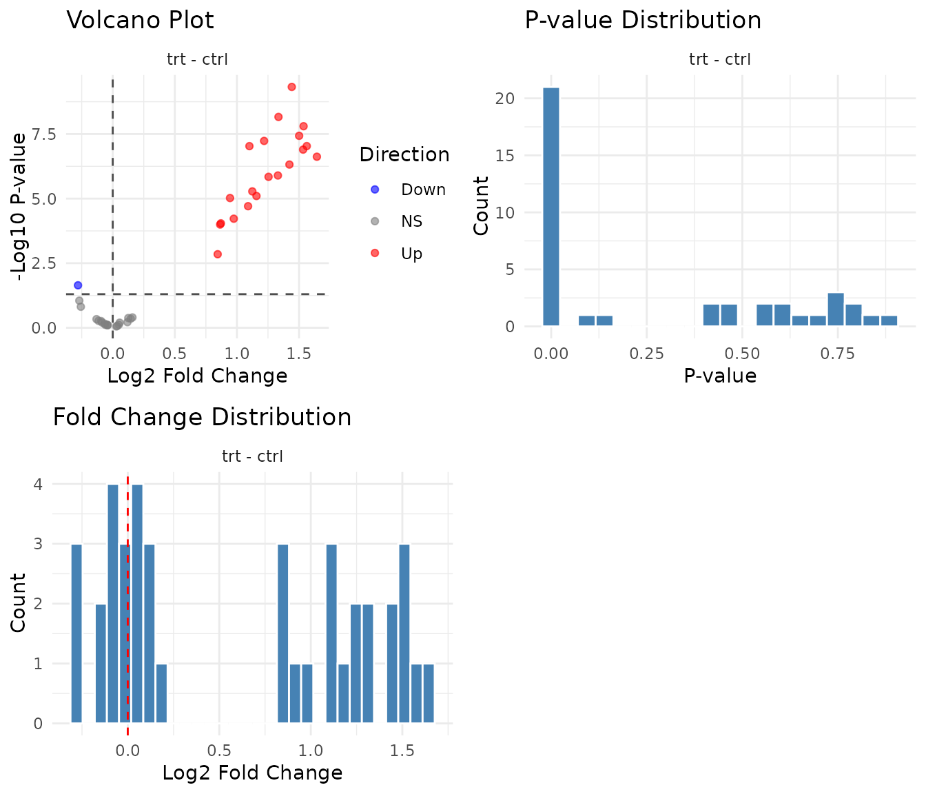

Stratified comparisons with within

The main effect averages across timepoints. But Group C has an effect at 24h only - the main effect diluted a 4-fold change to ~2-fold. Can we recover the true effect?

Use the within argument to get conditional effects - the treatment effect within each timepoint separately:

results_stratified <- compare(
  dat,
  compare = "treatment",
  ref = "ctrl",
  within = "timepoint",
  method = "glm"
)

results_stratified
#> pepdiff_results object
#> ----------------------
#> Method: glm
#> Peptides: 40
#> Comparisons: 1
#> Total tests: 80
#> 
#> Significant (FDR < 0.05): 30 (37.5%)
#> Marked significant: 30

Now we get separate comparisons: treatment effect at 0h, and treatment effect at 24h.

Stratified results by group

Let’s see how each group looks when we analyse timepoints separately:

results_stratified$results %>%
  mutate(
    pep_num = as.numeric(gsub("PEP_", "", peptide)),
    group = case_when(
      pep_num <= 10 ~ "A: Treatment only",
      pep_num <= 20 ~ "B: Timepoint only",
      pep_num <= 30 ~ "C: Interaction",
      TRUE ~ "D: No effect"
    )
  ) %>%
  group_by(group, timepoint) %>%
  summarise(
    n_significant = sum(significant),
    median_fc = round(median(fold_change, na.rm = TRUE), 2),
    .groups = "drop"
  ) %>%
  tidyr::pivot_wider(
    names_from = timepoint,
    values_from = c(n_significant, median_fc)
  )
#> # A tibble: 4 × 5
#>   group            n_significant_0h n_significant_24h median_fc_0h median_fc_24h
#>   <chr>                       <int>             <int>        <dbl>         <dbl>
#> 1 A: Treatment on…               10                10         2.6           2.86
#> 2 B: Timepoint on…                0                 0         0.99          0.94
#> 3 C: Interaction                  0                10         1.01          4.09
#> 4 D: No effect                    0                 0         1.01          0.96

What stratified analysis reveals:

• Group A: FC ≈ 3 at both timepoints — the main effect was accurate
• Group B: FC ≈ 1 at both timepoints, 0 significant — correctly negative at both
• Group C: FC ≈ 1 at 0h, FC ≈ 4 at 24h — now we see the true 4-fold effect!
• Group D: FC ≈ 1 at both, ~0 significant — correctly negative

For Group C, stratified analysis recovers the true 4-fold effect at 24h that was diluted to ~2-fold in the main effect.

Handling interactions

Group C illustrates an interaction: the treatment effect depends on timepoint. The main effect (FC ≈ 2) doesn’t represent either condition accurately - it’s the average of a 4-fold effect and no effect.

The emmeans warning: If you see “Results may be misleading due to involvement in interactions”, it means exactly this - the averaged main effect may not represent any real biological condition.

When to use main effects vs stratified

# Compare main vs stratified for all groups
main_summary <- results$results %>%
  mutate(
    pep_num = as.numeric(gsub("PEP_", "", peptide)),
    group = case_when(
      pep_num <= 10 ~ "A", pep_num <= 20 ~ "B",
      pep_num <= 30 ~ "C", TRUE ~ "D"
    )
  ) %>%
  group_by(group) %>%
  summarise(main_fc = round(median(fold_change, na.rm = TRUE), 2))

strat_summary <- results_stratified$results %>%
  mutate(
    pep_num = as.numeric(gsub("PEP_", "", peptide)),
    group = case_when(
      pep_num <= 10 ~ "A", pep_num <= 20 ~ "B",
      pep_num <= 30 ~ "C", TRUE ~ "D"
    )
  ) %>%
  group_by(group, timepoint) %>%
  summarise(fc = round(median(fold_change, na.rm = TRUE), 2), .groups = "drop") %>%
  tidyr::pivot_wider(names_from = timepoint, values_from = fc)

left_join(main_summary, strat_summary, by = "group")
#> # A tibble: 4 × 4
#>   group main_fc  `0h` `24h`
#>   <chr>   <dbl> <dbl> <dbl>
#> 1 A        2.77  2.6   2.86
#> 2 B        0.99  0.99  0.94
#> 3 C        2.05  1.01  4.09
#> 4 D        0.97  1.01  0.96

Use main effects when: the effect is consistent across conditions (Group A: ~3 at both timepoints, main ≈ 3)

Use stratified (within) when: the effect differs across conditions (Group C: ~1 at 0h, ~4 at 24h, main ≈ 2 is misleading)

Checking convergence

Not every peptide’s model will converge. This happens when: - Too few observations for that peptide - Extreme values or near-zero variance - Data patterns that the model can’t fit

# Check diagnostics
n_converged <- sum(results$diagnostics$converged)
n_failed <- sum(!results$diagnostics$converged)

cat("Converged:", n_converged, "\n")
#> Converged: 40
cat("Failed:", n_failed, "\n")
#> Failed: 0

Failed peptides are excluded from results. This is correct behaviour - if the model can’t fit, you shouldn’t trust its estimates.

# View failed peptides (if any)
results$diagnostics %>%
  filter(!converged) %>%
  select(peptide, converged)

Common causes of convergence failure: - Peptide measured in too few samples - All values identical (zero variance) - Extreme outliers - Too many missing values

What to do: - Check if failed peptides have data quality issues - Consider whether they have enough observations for the model complexity - Don’t force convergence - if it fails, you need more data or a simpler model - See peppwR for power analysis and sample size planning

Model checking

The diagnostics slot contains model information:

# Deviance: lower is better fit (relative to other peptides)
results$diagnostics %>%
  arrange(desc(deviance)) %>%
  head()
#> # A tibble: 6 × 7
#>   peptide converged error deviance residuals    std_residuals fitted      
#>   <chr>   <lgl>     <chr>    <dbl> <named list> <named list>  <named list>
#> 1 PEP_025 TRUE      NA        1.98 <dbl [20]>   <dbl [20]>    <dbl [20]>  
#> 2 PEP_015 TRUE      NA        1.89 <dbl [20]>   <dbl [20]>    <dbl [20]>  
#> 3 PEP_040 TRUE      NA        1.62 <dbl [20]>   <dbl [20]>    <dbl [20]>  
#> 4 PEP_019 TRUE      NA        1.42 <dbl [20]>   <dbl [20]>    <dbl [20]>  
#> 5 PEP_017 TRUE      NA        1.37 <dbl [20]>   <dbl [20]>    <dbl [20]>  
#> 6 PEP_008 TRUE      NA        1.34 <dbl [20]>   <dbl [20]>    <dbl [20]>

The error column contains diagnostic messages only when models fail to converge - NA means no error occurred (success). The deviance column measures model fit: high deviance relative to other peptides may indicate poor fit. Investigate these peptides if they’re in your significant results.

Exporting results

The results are stored in a tidy tibble, ready for export:

# Main effect results
glimpse(results$results)
#> Rows: 40
#> Columns: 11
#> $ peptide     <chr> "PEP_001", "PEP_002", "PEP_003", "PEP_004", "PEP_005", "PE…
#> $ gene_id     <chr> "GENE_A", "GENE_B", "GENE_C", "GENE_D", "GENE_E", "GENE_F"…
#> $ comparison  <chr> "trt - ctrl", "trt - ctrl", "trt - ctrl", "trt - ctrl", "t…
#> $ fold_change <dbl> 2.5219150, 2.9008270, 2.5137042, 3.1246797, 2.8298924, 2.3…
#> $ log2_fc     <dbl> 1.33451967, 1.53646428, 1.32981487, 1.64370830, 1.50074718…
#> $ estimate    <dbl> 0.92501854, 1.06499588, 0.92175743, 1.13933177, 1.04023868…
#> $ se          <dbl> 0.08385427, 0.10236298, 0.12294039, 0.13358011, 0.10630226…
#> $ test        <chr> "glm", "glm", "glm", "glm", "glm", "glm", "glm", "glm", "g…
#> $ p_value     <dbl> 6.895588e-09, 1.578496e-08, 1.273022e-06, 2.392305e-07, 3.…
#> $ fdr         <dbl> 1.379118e-07, 2.104661e-07, 4.629170e-06, 1.063247e-06, 3.…
#> $ significant <lgl> TRUE, TRUE, TRUE, TRUE, TRUE, TRUE, TRUE, TRUE, TRUE, TRUE…

Stratified results include the within factor as an additional column:

# Stratified results - note the timepoint column
glimpse(results_stratified$results)
#> Rows: 80
#> Columns: 13
#> $ peptide     <chr> "PEP_001", "PEP_002", "PEP_003", "PEP_004", "PEP_005", "PE…
#> $ gene_id     <chr> "GENE_A", "GENE_B", "GENE_C", "GENE_D", "GENE_E", "GENE_F"…
#> $ comparison  <chr> "trt - ctrl", "trt - ctrl", "trt - ctrl", "trt - ctrl", "t…
#> $ fold_change <dbl> 2.3064900, 2.6433935, 2.5347717, 3.2471510, 2.7527029, 2.5…
#> $ log2_fc     <dbl> 1.20569901, 1.40239120, 1.34185580, 1.69917447, 1.46084893…
#> $ estimate    <dbl> 0.83572687, 0.97206351, 0.93010356, 1.17777799, 1.01258332…
#> $ se          <dbl> 0.11726930, 0.16455790, 0.13108476, 0.22764781, 0.15943591…
#> $ test        <chr> "glm", "glm", "glm", "glm", "glm", "glm", "glm", "glm", "g…
#> $ p_value     <dbl> 9.935613e-05, 3.588548e-04, 1.024537e-04, 8.492950e-04, 2.…
#> $ fdr         <dbl> 0.0010245372, 0.0017942740, 0.0010245372, 0.0037746444, 0.…
#> $ significant <lgl> TRUE, TRUE, TRUE, TRUE, TRUE, TRUE, TRUE, TRUE, TRUE, TRUE…
#> $ stratum     <chr> "timepoint=0h", "timepoint=0h", "timepoint=0h", "timepoint…
#> $ timepoint   <chr> "0h", "0h", "0h", "0h", "0h", "0h", "0h", "0h", "0h", "0h"…

Save to CSV for downstream analysis:

# All results
write.csv(results$results, "glm_results.csv", row.names = FALSE)

# Significant hits only
results$results %>%
  filter(significant) %>%
  write.csv("significant_hits.csv", row.names = FALSE)

# Stratified results (one row per peptide per timepoint)
write.csv(results_stratified$results, "stratified_results.csv", row.names = FALSE)

Practical recommendations

1. Start simple: Run without within first to get main effects
2. Check for interactions: If effects differ across factor levels, use within (see below)
3. Inspect convergence: Many failures suggest the model is too complex for your data
4. Look at diagnostics: Volcano and p-value histogram should look reasonable
5. Don’t over-interpret: These are statistical estimates, not ground truth

Quick interaction check

To check for interactions in your own data, compare fold changes across strata:

compare(dat, compare = "treatment", ref = "ctrl",
        within = "timepoint", method = "glm")$results %>%
  group_by(timepoint) %>%
  summarise(median_fc = median(fold_change), .groups = "drop")

If these FCs differ substantially (e.g., 1 vs 4), you have an interaction - use stratified results.

When GLM struggles

• Very small sample sizes (< 3 per condition)
• Heavy-tailed or highly non-normal data
• Many zeros (consider whether these are true zeros or missing)

If GLM diagnostics look poor, try the ART method - see vignette("art_analysis").