Checking GLM Model Fit • pepdiff

library(pepdiff)
library(dplyr)

Why Check Model Fit?

pepdiff uses a Gamma GLM with log link for differential abundance analysis. This model assumes:

Abundances are positive (no zeros)
Variance increases with the mean (common in proteomics)
The relationship between predictors and response is multiplicative (log-linear)

When these assumptions hold, GLM gives reliable p-values and accurate fold change estimates. When they don’t, results may be misleading.

The good news: You don’t need a statistics degree to check model fit. plot_fit_diagnostics() gives you visual checks that tell you whether to trust your GLM results or try ART instead.

Quick Check with plot_fit_diagnostics()

Let’s start with simulated data that fits the GLM assumptions well.

set.seed(123)

n_peptides <- 40
n_reps <- 5

peptides <- paste0("PEP_", sprintf("%03d", 1:n_peptides))
genes <- paste0("GENE_", LETTERS[((1:n_peptides - 1) %% 26) + 1])

# Simulate well-behaved Gamma data
design <- expand.grid(
  peptide = peptides,
  treatment = c("ctrl", "trt"),
  bio_rep = 1:n_reps,
  stringsAsFactors = FALSE
)

sim_data <- design %>%
  mutate(
    gene_id = genes[match(peptide, peptides)],
    pep_num = as.numeric(gsub("PEP_", "", peptide)),
    base = 10 + pep_num * 0.5,
    # First 20 peptides have 2-fold treatment effect
    effect = ifelse(pep_num <= 20 & treatment == "trt", 2, 1),
    # Gamma noise (well-behaved)
    value = rgamma(n(), shape = 15, rate = 15 / (base * effect))
  ) %>%
  select(peptide, gene_id, treatment, bio_rep, value)

# Import
temp_file <- tempfile(fileext = ".csv")
write.csv(sim_data, temp_file, row.names = FALSE)

dat <- read_pepdiff(
  temp_file,
  id = "peptide",
  gene = "gene_id",
  value = "value",
  factors = "treatment",
  replicate = "bio_rep"
)

unlink(temp_file)

Run GLM analysis and check diagnostics:

results <- compare(dat, compare = "treatment", ref = "ctrl", method = "glm")

# Check fit diagnostics
diag <- plot_fit_diagnostics(results)
#> Warning in simpleLoess(y, x, w, span, degree = degree, parametric = parametric,
#> : pseudoinverse used at 11.91
#> Warning in simpleLoess(y, x, w, span, degree = degree, parametric = parametric,
#> : neighborhood radius 10.432
#> Warning in simpleLoess(y, x, w, span, degree = degree, parametric = parametric,
#> : reciprocal condition number 0
#> Warning in simpleLoess(y, x, w, span, degree = degree, parametric = parametric,
#> : There are other near singularities as well. 108.84
#> Warning in simpleLoess(y, x, w, span, degree = degree, parametric = parametric,
#> : pseudoinverse used at 10.412
#> Warning in simpleLoess(y, x, w, span, degree = degree, parametric = parametric,
#> : neighborhood radius 12.708
#> Warning in simpleLoess(y, x, w, span, degree = degree, parametric = parametric,
#> : reciprocal condition number 0
#> Warning in simpleLoess(y, x, w, span, degree = degree, parametric = parametric,
#> : There are other near singularities as well. 161.49
#> Warning in simpleLoess(y, x, w, span, degree = degree, parametric = parametric,
#> : pseudoinverse used at 16.759
#> Warning in simpleLoess(y, x, w, span, degree = degree, parametric = parametric,
#> : neighborhood radius 17.579
#> Warning in simpleLoess(y, x, w, span, degree = degree, parametric = parametric,
#> : reciprocal condition number 0
#> Warning in simpleLoess(y, x, w, span, degree = degree, parametric = parametric,
#> : There are other near singularities as well. 309.01
#> Warning in simpleLoess(y, x, w, span, degree = degree, parametric = parametric,
#> : pseudoinverse used at 21.973
#> Warning in simpleLoess(y, x, w, span, degree = degree, parametric = parametric,
#> : neighborhood radius 7.4351
#> Warning in simpleLoess(y, x, w, span, degree = degree, parametric = parametric,
#> : reciprocal condition number 0
#> Warning in simpleLoess(y, x, w, span, degree = degree, parametric = parametric,
#> : There are other near singularities as well. 55.281
#> Warning in simpleLoess(y, x, w, span, degree = degree, parametric = parametric,
#> : pseudoinverse used at 24.471
#> Warning in simpleLoess(y, x, w, span, degree = degree, parametric = parametric,
#> : neighborhood radius 3.7109
#> Warning in simpleLoess(y, x, w, span, degree = degree, parametric = parametric,
#> : reciprocal condition number 0
#> Warning in simpleLoess(y, x, w, span, degree = degree, parametric = parametric,
#> : There are other near singularities as well. 13.771
#> Warning in simpleLoess(y, x, w, span, degree = degree, parametric = parametric,
#> : pseudoinverse used at 26.085
#> Warning in simpleLoess(y, x, w, span, degree = degree, parametric = parametric,
#> : neighborhood radius 4.9087
#> Warning in simpleLoess(y, x, w, span, degree = degree, parametric = parametric,
#> : reciprocal condition number 0
#> Warning in simpleLoess(y, x, w, span, degree = degree, parametric = parametric,
#> : There are other near singularities as well. 24.095
#> 
#> GLM Fit Diagnostics
#> -------------------
#> Peptides analyzed: 40 (all converged)
#> Median deviance: 0.45
#> Threshold: 0.99 (95th percentile)
#> Flagged peptides: 2 (5.0%) above threshold
#> 
#> Interpretation: Some peptides show elevated deviance. Check residual plots.
#> See vignette('checking_fit') for detailed guidance.

diag$plot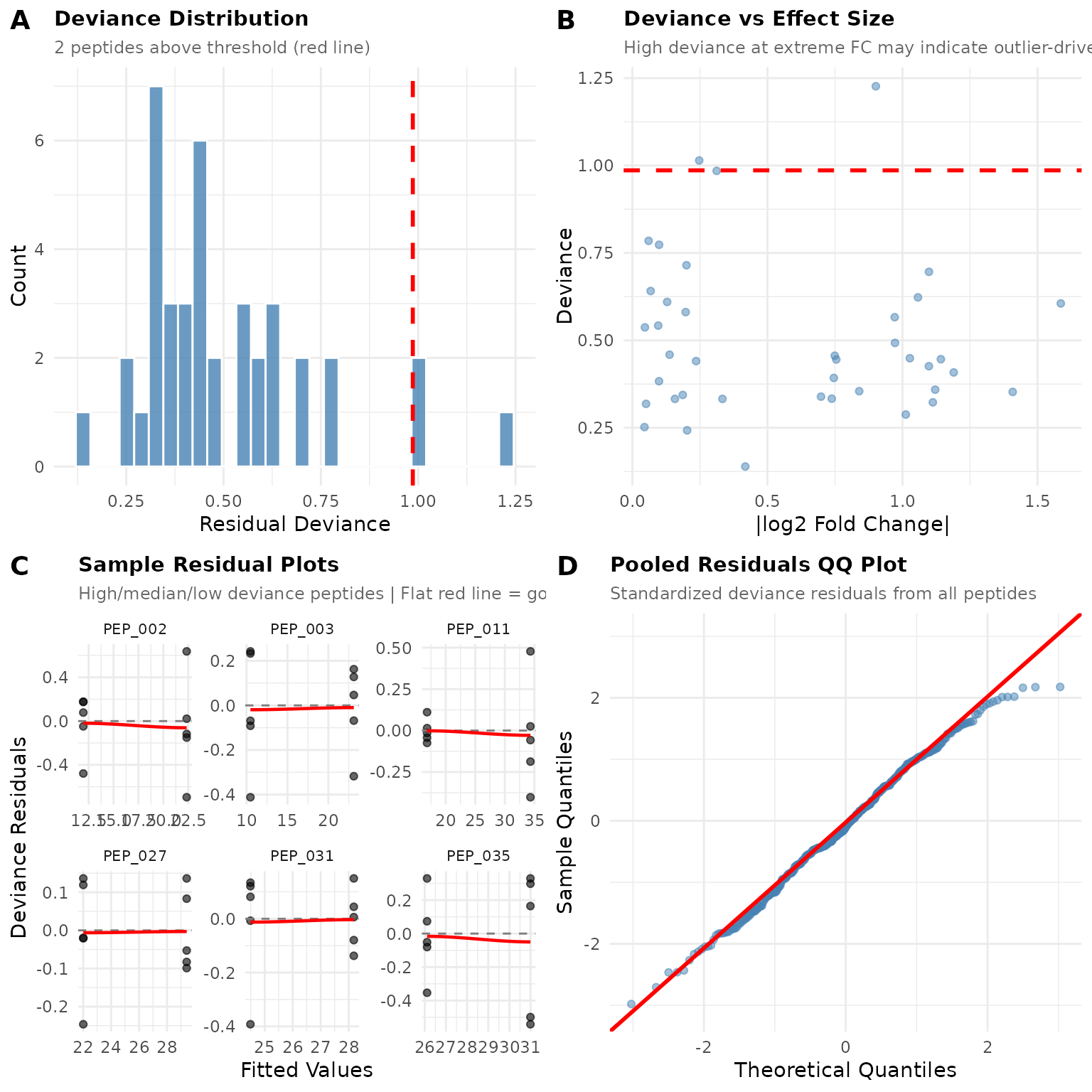

Reading the Diagnostic Plots

Panel A: Deviance Distribution

This histogram shows how well each peptide’s GLM model fits its data. Lower deviance = better fit.

What to look for: - Most peptides should cluster at low deviance values - A few peptides above the red threshold line is normal (by default, 5%) - A long right tail means some peptides fit poorly

In our example: The distribution is compact with only a few peptides above the threshold. This looks healthy.

Panel B: Deviance vs Effect Size

This scatter plot reveals whether poorly-fitting peptides cluster at certain effect sizes.

What to look for: - Random scatter = no systematic problem - High deviance at extreme fold changes = outlier-driven “significant” results (red flag) - Curved pattern = systematic misfit

In our example: Points are scattered without clear pattern. No obvious relationship between fold change and fit quality.

Panel C: Sample Residual Plots

These show residuals (observed - predicted) vs fitted values for individual peptides. The function selects peptides with high, median, and low deviance to give you a representative sample.

What good fit looks like: - Points scattered randomly around zero (the dashed line) - No funnel shape (variance shouldn’t change with fitted value) - Flat red loess line (no trend)

What poor fit looks like: - Curved pattern in points - Funnel shape (variance increasing or decreasing) - Curved red loess line

In our example: The residual plots show random scatter around zero with mostly flat loess lines.

Panel D: Pooled QQ Plot

This combines residuals from all peptides to check if they follow the expected distribution.

What good fit looks like: - Points fall along the diagonal line - Minor wiggles at the tails are OK

What poor fit looks like: - S-shaped curve = heavy tails (consider ART) - Systematic bow = wrong distributional assumption - Points far from line = outliers

In our example: Points follow the line reasonably well, suggesting the Gamma distribution is appropriate.

Investigating Flagged Peptides

The function identifies peptides with potential fit issues:

diag$flagged
#> # A tibble: 2 × 7
#>   peptide gene_id deviance fold_change p_value significant flag_reason  
#>   <chr>   <chr>      <dbl>       <dbl>   <dbl> <lgl>       <chr>        
#> 1 PEP_002 GENE_B      1.23        1.87  0.0330 FALSE       high_deviance
#> 2 PEP_035 GENE_I      1.01        1.19  0.441  FALSE       high_deviance

# Summary statistics
diag$summary
#> $n_analyzed
#> [1] 40
#> 
#> $n_converged
#> [1] 40
#> 
#> $n_failed
#> [1] 0
#> 
#> $median_deviance
#> [1] 0.4457115
#> 
#> $threshold
#>      95% 
#> 0.986245 
#> 
#> $n_flagged
#> [1] 2
#> 
#> $pct_flagged
#> [1] 5

If peptides are flagged, investigate them:

Check the data - Do these peptides have outliers, zeros, or unusual patterns?
Look at sample size - Low replication can cause fitting issues
Consider biology - Are these peptides biologically different?

Example: Data with Poor Fit

Let’s simulate data that violates GLM assumptions - heavy tails with outliers:

set.seed(456)

# Same design but with outliers and heavy tails
sim_bad <- design %>%
  mutate(
    gene_id = genes[match(peptide, peptides)],
    pep_num = as.numeric(gsub("PEP_", "", peptide)),
    base = 10 + pep_num * 0.5,
    effect = ifelse(pep_num <= 20 & treatment == "trt", 2, 1),
    # Add outliers (10% of observations)
    outlier = ifelse(runif(n()) < 0.1, runif(n(), 3, 8), 1),
    # Heavier-tailed noise
    value = rgamma(n(), shape = 3, rate = 3 / (base * effect)) * outlier
  ) %>%
  select(peptide, gene_id, treatment, bio_rep, value)

temp_file <- tempfile(fileext = ".csv")
write.csv(sim_bad, temp_file, row.names = FALSE)

dat_bad <- read_pepdiff(
  temp_file,
  id = "peptide",
  gene = "gene_id",
  value = "value",
  factors = "treatment",
  replicate = "bio_rep"
)

unlink(temp_file)

results_bad <- compare(dat_bad, compare = "treatment", ref = "ctrl", method = "glm")
diag_bad <- plot_fit_diagnostics(results_bad)
#> Warning in simpleLoess(y, x, w, span, degree = degree, parametric = parametric,
#> : pseudoinverse used at 21.493
#> Warning in simpleLoess(y, x, w, span, degree = degree, parametric = parametric,
#> : neighborhood radius 27.638
#> Warning in simpleLoess(y, x, w, span, degree = degree, parametric = parametric,
#> : reciprocal condition number 0
#> Warning in simpleLoess(y, x, w, span, degree = degree, parametric = parametric,
#> : There are other near singularities as well. 763.86
#> Warning in simpleLoess(y, x, w, span, degree = degree, parametric = parametric,
#> : pseudoinverse used at 14.896
#> Warning in simpleLoess(y, x, w, span, degree = degree, parametric = parametric,
#> : neighborhood radius 12.748
#> Warning in simpleLoess(y, x, w, span, degree = degree, parametric = parametric,
#> : reciprocal condition number 0
#> Warning in simpleLoess(y, x, w, span, degree = degree, parametric = parametric,
#> : There are other near singularities as well. 162.51
#> Warning in simpleLoess(y, x, w, span, degree = degree, parametric = parametric,
#> : pseudoinverse used at 14.22
#> Warning in simpleLoess(y, x, w, span, degree = degree, parametric = parametric,
#> : neighborhood radius 19.399
#> Warning in simpleLoess(y, x, w, span, degree = degree, parametric = parametric,
#> : reciprocal condition number 0
#> Warning in simpleLoess(y, x, w, span, degree = degree, parametric = parametric,
#> : There are other near singularities as well. 376.31
#> Warning in simpleLoess(y, x, w, span, degree = degree, parametric = parametric,
#> : pseudoinverse used at 34.436
#> Warning in simpleLoess(y, x, w, span, degree = degree, parametric = parametric,
#> : neighborhood radius 2.2455
#> Warning in simpleLoess(y, x, w, span, degree = degree, parametric = parametric,
#> : reciprocal condition number 0
#> Warning in simpleLoess(y, x, w, span, degree = degree, parametric = parametric,
#> : There are other near singularities as well. 5.0422
#> Warning in simpleLoess(y, x, w, span, degree = degree, parametric = parametric,
#> : pseudoinverse used at 25.642
#> Warning in simpleLoess(y, x, w, span, degree = degree, parametric = parametric,
#> : neighborhood radius 11.877
#> Warning in simpleLoess(y, x, w, span, degree = degree, parametric = parametric,
#> : reciprocal condition number 0
#> Warning in simpleLoess(y, x, w, span, degree = degree, parametric = parametric,
#> : There are other near singularities as well. 141.07
#> Warning in simpleLoess(y, x, w, span, degree = degree, parametric = parametric,
#> : pseudoinverse used at 23.201
#> Warning in simpleLoess(y, x, w, span, degree = degree, parametric = parametric,
#> : neighborhood radius 31.311
#> Warning in simpleLoess(y, x, w, span, degree = degree, parametric = parametric,
#> : reciprocal condition number 0
#> Warning in simpleLoess(y, x, w, span, degree = degree, parametric = parametric,
#> : There are other near singularities as well. 980.4
#> 
#> GLM Fit Diagnostics
#> -------------------
#> Peptides analyzed: 40 (all converged)
#> Median deviance: 4.97
#> Threshold: 9.89 (95th percentile)
#> Flagged peptides: 2 (5.0%) above threshold
#> 
#> Interpretation: Some peptides show elevated deviance. Check residual plots.
#> See vignette('checking_fit') for detailed guidance.

diag_bad$plot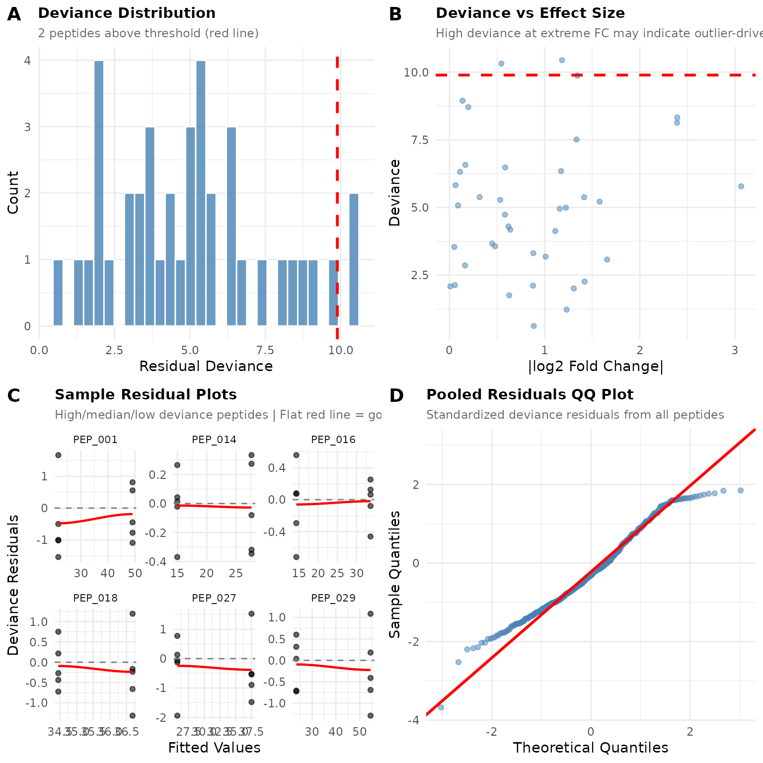

Notice the differences:

Deviance distribution has a longer right tail with more flagged peptides
Residual plots may show non-random patterns
QQ plot deviates from the line, especially in the tails

When diagnostics look like this, ART may be more appropriate.

Decision: GLM or ART?

Use GLM when:

Deviance distribution looks reasonable (few flagged, <10-15%)
No systematic patterns in residual plots
QQ plot is reasonably linear
You want interpretable fold changes

Consider ART when:

Many peptides (>15%) have high deviance
Residual plots show systematic curves or funnels
QQ plot shows heavy tails (S-curve)
You have known outliers or heavy-tailed data
You’re uncomfortable with distributional assumptions

Try ART on the problematic data:

results_art <- compare(dat_bad, compare = "treatment", ref = "ctrl", method = "art")

# Compare significant calls
comparison <- tibble(
  peptide = results_bad$results$peptide,
  glm_sig = results_bad$results$significant,
  art_sig = results_art$results$significant
)

cat("Both significant:", sum(comparison$glm_sig & comparison$art_sig), "\n")
#> Both significant: 0
cat("GLM only:", sum(comparison$glm_sig & !comparison$art_sig), "\n")
#> GLM only: 0
cat("ART only:", sum(!comparison$glm_sig & comparison$art_sig), "\n")
#> ART only: 5

Summary

Always run plot_fit_diagnostics() after GLM analysis - it only takes seconds
Check all four panels for warning signs
Investigate flagged peptides if needed - check for data quality issues
Switch to ART only if diagnostics suggest systematic problems - ART trades power for robustness
When in doubt, run both methods and compare results

GLM is the default because it’s more powerful when assumptions hold. Use diagnostics to verify those assumptions, and switch to ART when they don’t.

See vignette("art_analysis") for details on using the ART method.