Non-parametric Factorial Analysis with ART
art_analysis.RmdWhat is ART?
ART (Aligned Rank Transform) is a non-parametric method for factorial designs. It lets you analyse multi-factor experiments without assuming your data follows a particular distribution.
The problem it solves: Wilcoxon and other rank tests work great for two groups, but can’t handle interactions. Parametric ANOVA handles interactions but assumes normality. ART gives you both: non-parametric robustness with factorial capability.
How it works: 1. Align: Subtract out all effects except the one you’re testing, so residuals reflect only that effect 2. Rank: Convert aligned values to ranks 3. ANOVA: Run standard ANOVA on the ranks
The alignment step is crucial - it allows the test to isolate each effect (main effects, interactions) correctly.
When to consider ART
- GLM fit diagnostics show problems (see
vignette("checking_fit")) - Heavy-tailed data with extreme values
- You’re uncomfortable with distributional assumptions
- Ordinal data that doesn’t meet interval scale assumptions
Requirements:
- Balanced-ish designs work best
- Complete cases for each peptide
Example: 2×2 factorial design
A 2×2 factorial design means two factors, each with two levels. Here: treatment (ctrl, trt) × timepoint (early, late). This gives four experimental conditions:
| early | late | |
|---|---|---|
| ctrl | ✓ | ✓ |
| trt | ✓ | ✓ |
Each peptide is measured in all four conditions (with replicates), letting us ask: does treatment have an effect? Does that effect depend on timepoint?
We’ll use 5 replicates per condition and simulate data with heavy tails (extreme values) - exactly the scenario where ART shines.
The simulated peptide groups
To illustrate how ART handles different effect patterns, we simulate 40 peptides in four groups:
| Group | Peptides | Effect Pattern | What ART should find |
|---|---|---|---|
| A | PEP_001–010 | Treatment effect only | Main effect significant, same at both timepoints |
| B | PEP_011–020 | Timepoint effect only | No treatment effect (treatment comparison) |
| C | PEP_021–030 | Interaction | Treatment works at late but not early |
| D | PEP_031–040 | No effect | Nothing significant |
What these patterns look like in raw data
Here’s what the mean abundances look like for each group across the four conditions (using a baseline of ~10 for illustration):
| Group | ctrl @ early | ctrl @ late | trt @ early | trt @ late | Pattern |
|---|---|---|---|---|---|
| A | 10 | 10 | 30 | 30 | trt 3× higher at both timepoints |
| B | 10 | 30 | 10 | 30 | late 3× higher, same for ctrl and trt |
| C | 10 | 10 | 10 | 40 | trt effect only at late (interaction) |
| D | 10 | 10 | 10 | 10 | no differences |
Notice how Group C is the tricky one: treatment has no effect at early (10 vs 10) but a 4-fold effect at late (10 vs 40). The main effect would average these, giving ~2-fold - which doesn’t represent either timepoint accurately.
We’ll refer back to these groups as we analyse the results.
set.seed(789)

n_peptides <- 40
n_reps <- 5  # 5 reps per condition = 20 observations per peptide

peptides <- paste0("PEP_", sprintf("%03d", 1:n_peptides))
genes <- paste0("GENE_", LETTERS[((1:n_peptides - 1) %% 26) + 1])

# Step 1: Create base abundance for each peptide
peptide_info <- tibble(

  peptide = peptides,
  gene_id = genes,
  pep_num = 1:n_peptides,
  base = rgamma(n_peptides, shape = 6, rate = 0.6)
)

# Step 2: Create the experimental design
design <- expand.grid(
  peptide = peptides,
  treatment = c("ctrl", "trt"),
  timepoint = c("early", "late"),
  bio_rep = 1:n_reps,
  stringsAsFactors = FALSE
)

# Step 3: Join design with peptide info and apply effects
# Using heavier-tailed noise to justify ART
sim_data <- design %>%
  left_join(peptide_info, by = "peptide") %>%
  mutate(
    # Group A (peptides 1-10): Treatment effect only
    # trt is 3-fold higher than ctrl, same at both timepoints
    trt_effect = ifelse(pep_num <= 10 & treatment == "trt", 3, 1),

    # Group B (peptides 11-20): Timepoint effect only
    # late is 3-fold higher than early, same for both treatments
    time_effect = ifelse(pep_num > 10 & pep_num <= 20 & timepoint == "late", 3, 1),

    # Group C (peptides 21-30): Interaction
    # Treatment works at late (4-fold) but NOT at early
    int_effect = case_when(
      pep_num > 20 & pep_num <= 30 & treatment == "trt" & timepoint == "late" ~ 4,
      TRUE ~ 1
    ),

    # Group D (peptides 31-40): No effect
    # All effect multipliers are 1

    # Add heavy-tailed noise (occasional extreme values)
    # This is why we might prefer ART over GLM
    extreme = ifelse(runif(n()) < 0.05, runif(n(), 2, 4), 1),

    # Final abundance with Gamma noise and occasional extremes
    value = rgamma(n(), shape = 10, rate = 10 / (base * trt_effect * time_effect * int_effect)) * extreme
  ) %>%
  select(peptide, gene_id, treatment, timepoint, bio_rep, value)

# Import
temp_file <- tempfile(fileext = ".csv")
write.csv(sim_data, temp_file, row.names = FALSE)

dat <- read_pepdiff(
  temp_file,
  id = "peptide",
  gene = "gene_id",
  value = "value",
  factors = c("treatment", "timepoint"),
  replicate = "bio_rep"
)

dat
#> pepdiff_data object
#> -------------------
#> Peptides: 40
#> Observations: 800
#> Factors: treatment, timepoint
#>
#> Design:
#>   treatment=ctrl, timepoint=early: 5 reps
#>   treatment=ctrl, timepoint=late: 5 reps
#>   treatment=trt, timepoint=early: 5 reps
#>   treatment=trt, timepoint=late: 5 reps
#>
#> No missing values
Running ART analysis
results_art <- compare(
  dat,
  compare = "treatment",
  ref = "ctrl",
  method = "art"
)

results_art
#> pepdiff_results object
#> ----------------------
#> Method: art
#> Peptides: 40
#> Comparisons: 1
#> Total tests: 40
#>
#> Significant (FDR < 0.05): 20 (50.0%)
#> Marked significant: 20
The interface is identical to GLM - just change
method = "art".
Did ART find the treatment effects?
Since we simulated this data, we know the truth:
- Group A: 3-fold treatment effect at both timepoints
- Group B: No treatment effect (the timepoint change affects ctrl and trt equally)
- Group C: 4-fold treatment effect at late, but no effect at early
- Group D: No effect
Let’s see what ART finds:
results_art$results %>%
  mutate(
    pep_num = as.numeric(gsub("PEP_", "", peptide)),
    group = case_when(
      pep_num <= 10 ~ "A: Treatment only",
      pep_num <= 20 ~ "B: Timepoint only",
      pep_num <= 30 ~ "C: Interaction",
      TRUE ~ "D: No effect"
    )
  ) %>%
  group_by(group) %>%
  summarise(
    n_significant = sum(significant),
    n_peptides = n(),
    median_fc = round(median(fold_change, na.rm = TRUE), 2)
  )
#> # A tibble: 4 × 4
#>   group             n_significant n_peptides median_fc
#>   <chr>                     <int>      <int>     <dbl>
#> 1 A: Treatment only            10         10      2.75
#> 2 B: Timepoint only             0         10      0.92
#> 3 C: Interaction               10         10      2.31
#> 4 D: No effect 0 10 1.1- Group A: Treatment effect detected ✓
- Group B: Correctly negative (no treatment effect) ✓
- Group C: Detected, but note the diluted fold change (~2 instead of 4) - the main effect averages across timepoints
- Group D: Correctly negative ✓
plot(results_art)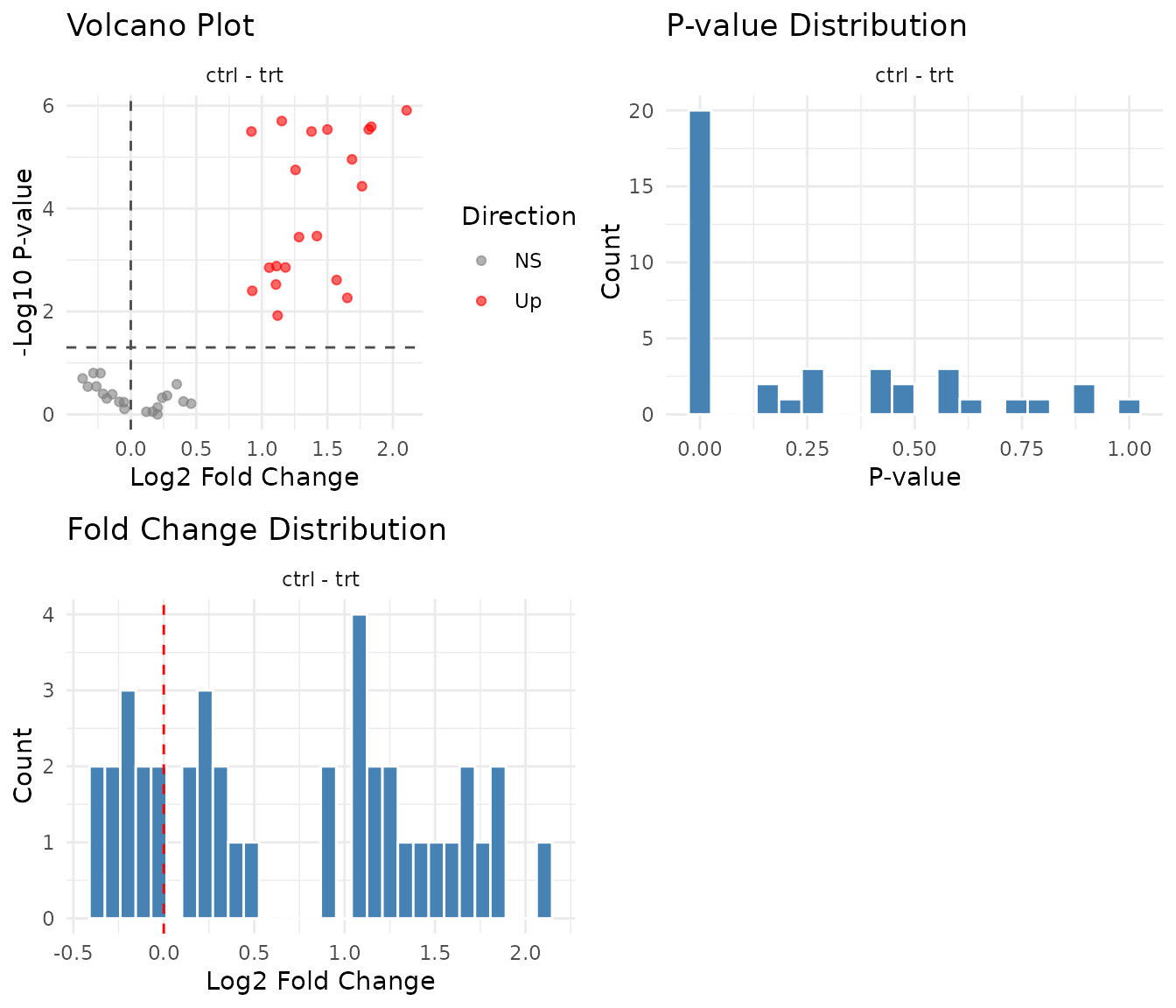
Stratified comparisons with within
Just like GLM, use within to get treatment effects at
each timepoint separately:
results_strat <- compare(
  dat,
  compare = "treatment",
  ref = "ctrl",
  within = "timepoint",
  method = "art"
)

results_strat
#> pepdiff_results object
#> ----------------------
#> Method: art
#> Peptides: 40
#> Comparisons: 1
#> Total tests: 80
#>
#> Significant (FDR < 0.05): 26 (32.5%)
#> Marked significant: 26
Stratified results by group
Let’s see how each group looks when we analyse timepoints separately:
results_strat$results %>%
  mutate(
    pep_num = as.numeric(gsub("PEP_", "", peptide)),
    group = case_when(
      pep_num <= 10 ~ "A: Treatment only",
      pep_num <= 20 ~ "B: Timepoint only",
      pep_num <= 30 ~ "C: Interaction",
      TRUE ~ "D: No effect"
    )
  ) %>%
  group_by(group, timepoint) %>%
  summarise(
    n_significant = sum(significant),
    median_fc = round(median(fold_change, na.rm = TRUE), 2),
    .groups = "drop"
  ) %>%
  tidyr::pivot_wider(
    names_from = timepoint,
    values_from = c(n_significant, median_fc)
  )
#> # A tibble: 4 × 5
#>   group    n_significant_early n_significant_late median_fc_early median_fc_late
#>   <chr>                  <int>              <int>           <dbl>          <dbl>
#> 1 A: Trea…                   7                  8            3.31           2.67
#> 2 B: Time…                   1                  0            0.87           0.96
#> 3 C: Inte…                   0                 10            0.95           3.63
#> 4 D: No e…                   0                  0            1.24           0.97
What stratified analysis reveals:
- Group A: FC ≈ 3 at both timepoints — the main effect was accurate
- Group B: FC ≈ 1 at both timepoints, 0 significant — correctly negative at both
- Group C: FC ≈ 1 at early, FC ≈ 4 at late — now we see the true effect!
- Group D: FC ≈ 1 at both, ~0 significant — correctly negative
For Group C, stratified analysis recovers the true 4-fold effect at late that was diluted in the main effect.
Handling interactions
Group C illustrates an interaction: the treatment
effect depends on timepoint. ART handles this the same way as GLM - use
within to get conditional effects at each level.
For more details on interpreting interactions, see
vignette("glm_analysis").
ART vs GLM comparison
Let’s compare both methods on the same data:
results_glm <- compare(dat, compare = "treatment", ref = "ctrl", method = "glm")
# Compare significant calls
comparison <- tibble(
  peptide = results_glm$results$peptide,
  glm_sig = results_glm$results$significant,
  art_sig = results_art$results$significant,
  glm_pval = round(results_glm$results$p_value, 4),
  art_pval = round(results_art$results$p_value, 4)
)

# Agreement
cat("Both significant:", sum(comparison$glm_sig & comparison$art_sig), "\n")
#> Both significant: 19
cat("GLM only:", sum(comparison$glm_sig & !comparison$art_sig), "\n")
#> GLM only: 1
cat("ART only:", sum(!comparison$glm_sig & comparison$art_sig), "\n")
#> ART only: 1
cat("Neither:", sum(!comparison$glm_sig & !comparison$art_sig), "\n")
#> Neither: 19
When both methods agree, you can be confident in the result. When they disagree, investigate the peptide:
# Peptides where methods disagree
disagreements <- comparison %>%
  filter(glm_sig != art_sig) %>%
  arrange(pmin(glm_pval, art_pval))

if (nrow(disagreements) > 0) {
  print(disagreements)
} else {
  cat("No disagreements between methods\n")
}
#> # A tibble: 2 × 5
#>   peptide glm_sig art_sig glm_pval art_pval
#>   <chr>   <lgl>   <lgl>      <dbl>    <dbl>
#> 1 PEP_022 FALSE   TRUE      0.0363    0.004
#> 2 PEP_016 TRUE    FALSE     0.0128    0.158
Diagnostics
results_art$diagnostics %>%
  head()
#> # A tibble: 6 × 7
#>   peptide converged error deviance residuals    std_residuals fitted
#>   <chr>   <lgl>     <chr>    <dbl> <named list> <named list>  <named list>
#> 1 PEP_001 TRUE      NA          NA <dbl [20]>   <NULL>        <NULL>
#> 2 PEP_002 TRUE      NA          NA <dbl [20]>   <NULL>        <NULL>
#> 3 PEP_003 TRUE      NA          NA <dbl [20]>   <NULL>        <NULL>
#> 4 PEP_004 TRUE      NA          NA <dbl [20]>   <NULL>        <NULL>
#> 5 PEP_005 TRUE      NA          NA <dbl [20]>   <NULL>        <NULL>
#> 6 PEP_006 TRUE      NA          NA <dbl [20]>   <NULL>        <NULL>
The error column contains diagnostic messages only when
models fail - NA means success. Check convergence:
n_converged <- sum(results_art$diagnostics$converged)
n_failed <- sum(!results_art$diagnostics$converged)

cat("Converged:", n_converged, "\n")
#> Converged: 40
cat("Failed:", n_failed, "\n")
#> Failed: 0
The same diagnostic plots apply:
- Volcano should be symmetric
- P-value histogram should show uniform + spike pattern
- Fold change distribution should centre near zero
Exporting results
The results are stored in a tidy tibble:
glimpse(results_art$results)
#> Rows: 40
#> Columns: 11
#> $ peptide     <chr> "PEP_001", "PEP_002", "PEP_003", "PEP_004", "PEP_005", "PE…
#> $ gene_id     <chr> "GENE_A", "GENE_B", "GENE_C", "GENE_D", "GENE_E", "GENE_F"…
#> $ comparison  <chr> "ctrl - trt", "ctrl - trt", "ctrl - trt", "ctrl - trt", "c…
#> $ fold_change <dbl> 2.2658580, 3.5678933, 3.5203738, 2.6765771, 4.3006451, 2.8…
#> $ log2_fc     <dbl> 1.18005748, 1.83507248, 1.81572864, 1.42038920, 2.10455309…
#> $ estimate    <dbl> -8.00000e+00, -1.00000e+01, -1.00000e+01, -8.60000e+00, -1…
#> $ se          <dbl> 2.073644, 1.410674, 1.424781, 1.898684, 1.330413, 1.424781…
#> $ test        <chr> "art", "art", "art", "art", "art", "art", "art", "art", "a…
#> $ p_value     <dbl> 1.391822e-03, 2.565233e-06, 2.899704e-06, 3.420731e-04, 1.…
#> $ fdr         <dbl> 3.746732e-03, 1.812999e-05, 1.812999e-05, 1.192848e-03, 1.…
#> $ significant <lgl> TRUE, TRUE, TRUE, TRUE, TRUE, TRUE, TRUE, TRUE, TRUE, TRUE…
Stratified results include the timepoint column:
glimpse(results_strat$results)
#> Rows: 80
#> Columns: 13
#> $ peptide     <chr> "PEP_001", "PEP_002", "PEP_003", "PEP_004", "PEP_005", "PE…
#> $ gene_id     <chr> "GENE_A", "GENE_B", "GENE_C", "GENE_D", "GENE_E", "GENE_F"…
#> $ comparison  <chr> "ctrl - trt", "ctrl - trt", "ctrl - trt", "ctrl - trt", "c…
#> $ fold_change <dbl> 2.5351923, 4.3127474, 3.8037220, 3.6106241, 5.5918984, 3.0…
#> $ log2_fc     <dbl> 1.342095192, 2.108607216, 1.927411826, 1.852248235, 2.4833…
#> $ estimate    <dbl> -3.8, -5.0, -5.0, -5.0, -5.0, -5.0, -5.0, -3.8, -3.0, -5.0…
#> $ se          <dbl> 1.523155, 1.000000, 1.000000, 1.000000, 1.000000, 1.000000…
#> $ test        <chr> "art", "art", "art", "art", "art", "art", "art", "art", "a…
#> $ p_value     <dbl> 0.037241306, 0.001052826, 0.001052826, 0.001052826, 0.0010…
#> $ fdr         <dbl> 0.148965224, 0.006016147, 0.006016147, 0.006016147, 0.0060…
#> $ significant <lgl> FALSE, TRUE, TRUE, TRUE, TRUE, TRUE, TRUE, FALSE, FALSE, T…
#> $ stratum     <chr> "timepoint=early", "timepoint=early", "timepoint=early", "…
#> $ timepoint   <chr> "early", "early", "early", "early", "early", "early", "ear…
Save to CSV for downstream analysis:
# All results
write.csv(results_art$results, "art_results.csv", row.names = FALSE)

# Significant hits only
results_art$results %>%
  filter(significant) %>%
  write.csv("art_significant.csv", row.names = FALSE)

# Stratified results
write.csv(results_strat$results, "art_stratified.csv", row.names = FALSE)
Limitations of ART
Speed: ART is slower than GLM because it fits multiple aligned models per peptide. For large datasets, this matters.
Interpretation: Rank-based effects are less intuitive than fold changes. “Treatment increases ranks” is harder to communicate than “treatment doubles abundance”.
Balance: ART works best with balanced designs (equal n per cell). Unbalanced designs can give unreliable interaction tests.
Not a magic fix: If your data has fundamental problems (outlier samples, batch effects), ART won’t save you. Fix the problems first.
Practical recommendations
- Start with GLM - it’s the default for good reason
-
Check GLM fit - run
plot_fit_diagnostics(results)(seevignette("checking_fit")) - If diagnostics look poor, try ART on the same data
- Compare results - where do methods agree and disagree?
- For publication, report which method you used and why
Decision tree:
GLM diagnostics OK?
  → Yes: Use GLM
  → No: Try ART
         ↓
       ART diagnostics OK?
         → Yes: Use ART
         → No: You may need more data, or the effect isn't there
When both methods fail
If neither GLM nor ART gives sensible results:
- Check data quality: Outlier samples, batch effects, normalisation issues
- Consider sample size: May not have power to detect effects
- Simplify the model: Too many factors for the data?
- Accept the null: Sometimes there’s no effect to find
See peppwR for power analysis to understand what effect sizes your experiment can detect.