Power Analysis for Targeted Proteomics with Missing Data (PRM)
peppwR
2026-04-16
Source:vignettes/articles/prm-genotype-power.Rmd
prm-genotype-power.RmdIntroduction
What Makes Targeted Proteomics Different?
Targeted proteomics (PRM/SRM) takes aim at specific targets:
- Measures a pre-defined panel of peptides
- Higher sensitivity and reproducibility
- Better for hypothesis testing
- Lower multiple testing burden
This document analyzes a PRM dataset, demonstrating how peppwR handles the unique challenges of targeted proteomics, including missing data and FDR considerations.
The Missing Data Challenge
Even with targeted methods, missing values are ubiquitous in mass spectrometry. But not all missing data is created equal:
MCAR (Missing Completely At Random)
- Values missing due to random technical failures
- No relationship to abundance
- Reduces sample size but doesn’t bias results
MNAR (Missing Not At Random)
- Low-abundance peptides systematically missing
- Below detection limit = no measurement
- Can bias abundance estimates upward
- Common in mass spectrometry
peppwR tracks both the rate of missingness AND evidence for MNAR patterns, enabling more realistic power estimates.
About the Data
This analysis uses fungal phosphoproteomics data from a targeted PRM experiment:
| Property | Value |
|---|---|
| Organism | Magnaporthe oryzae (rice blast fungus) |
| Method | PRM (Parallel Reaction Monitoring) |
| Comparison | Early (t=0) vs late (t=6) timepoints |
| Biological replicates | 3 per condition |
| Technical replicates | 2 per biological replicate |
| Peptides | 285 phosphopeptides |
| Missing data | ~17% |
Data Preparation
# Load the PRM experiment data
prm <- read.csv("../../sample_data/prm_data.csv")

# Examine the structure
glimpse(prm)
## Rows: 20,520
## Columns: 7
## $ molecule_list_name <chr> "MOL_0001", "MOL_0001", "MOL_0001", "MOL_000…
## $ peptide_modified_sequence <chr> "PEP_00001", "PEP_00001", "PEP_00001", "PEP_…
## $ genotype <chr> "Genotype_A", "Genotype_A", "Genotype_A", "G…
## $ timepoint <dbl> 0.0, 0.0, 0.0, 0.0, 0.0, 0.0, 1.0, 1.0, 1.0,…
## $ bio_rep <int> 1, 1, 2, 2, 3, 3, 1, 1, 2, 2, 3, 3, 1, 1, 2,…
## $ tech_rep <int> 1, 2, 1, 2, 1, 2, 1, 2, 1, 2, 1, 2, 1, 2, 1,…
## $ total_area <dbl> 1.031275e-03, 1.130267e-03, 5.243216e-04, 2.…## Total observations: 20520## Missing values: 3547## Missing rate: 17.3 %Why Average Technical Replicates?
Technical replicates measure the same biological sample multiple times. They capture measurement variability, not biological variability.
For power analysis, biological replicates are the true unit of replication - they represent independent observations of the biological phenomenon we’re studying. We average technical replicates to get one value per biological replicate.
# Filter to early (0) vs late (6) timepoints
# Average technical replicates within each biological replicate
pilot <- prm |>
  filter(timepoint %in% c(0, 6)) |>
  group_by(peptide_modified_sequence, genotype, timepoint, bio_rep) |>
  summarise(abundance = mean(total_area, na.rm = TRUE), .groups = "drop") |>
  transmute(
    peptide_id = peptide_modified_sequence,
    condition = paste0("t", timepoint),
    abundance = abundance
  )

# Summary statistics
cat("Unique peptides:", n_distinct(pilot$peptide_id), "\n")
## Unique peptides: 285
cat("Observations per condition:\n")## Observations per condition:
pilot |> count(condition)## # A tibble: 2 × 2
## condition n
## <chr> <int>
## 1 t0 1710
## 2 t6 1710
# Check missingness after averaging technical replicates
# (NaN results when both tech reps are NA)
pilot <- pilot |>
  mutate(abundance = ifelse(is.nan(abundance), NA, abundance))

cat("Missing after averaging tech reps:", sum(is.na(pilot$abundance)), "\n")
## Missing after averaging tech reps: 429## Missing rate: 12.5 %Missingness Analysis
Examining the Extent of Missingness
Before diving into power analysis, we need to understand our missing data. peppwR automatically computes missingness statistics during distribution fitting.
# Fit distributions - missingness is tracked automatically
fits <- fit_distributions(pilot, "peptide_id", "condition", "abundance")

# Summary includes missingness information
print(fits)
## peppwr_fits object
## ------------------
## 570 peptides fitted
##
## Best fit distribution counts:
## Gamma: 103
## Inverse Gaussian: 36
## InvGamma: 2
## Lognormal: 5
## Normal: 91
## Pareto: 273
## Skew Normal: 60
##
## Missingness: 429/3420 values NA (12.5%)
## Peptides with missing data: 180
##
## MNAR detection (abundance vs missingness):
## Correlation: r = -0.40 (p = 1.3e-07)
## Moderate evidence of MNAR: low-abundance peptides have more missing values (p = 1.3e-07)Visualizing Missingness Patterns
The plot_missingness() function provides three
complementary views:
- NA Rate Distribution: What fraction of observations are missing for each peptide?
- Abundance vs NA Rate: Do low-abundance peptides have more missing values?
plot_missingness(fits)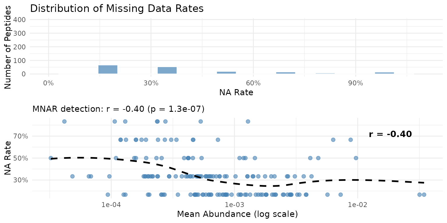
Missingness patterns across the PRM peptidome. Left: Distribution of NA rates. Right: Relationship between mean abundance and NA rate.
MNAR Detection
MNAR (Missing Not At Random) in mass spectrometry typically occurs when low-abundance peptides fall below the detection limit. peppwR detects this by correlating mean abundance with NA rate across all peptides.
A negative correlation indicates that low-abundance peptides have more missing values - the hallmark of detection-limit-driven missingness.
| Correlation (r) | Interpretation |
|---|---|
| r > -0.1 | No evidence of MNAR |
| -0.3 < r < -0.1 | Weak evidence of MNAR |
| -0.5 < r < -0.3 | Moderate evidence of MNAR |
| r < -0.5 | Strong evidence of MNAR |
Implications of MNAR
When MNAR is detected, be aware that:
- Abundance estimates for low-abundance peptides may be biased upward (since low values are missing)
- Power calculations may be optimistic for these peptides
- Consider robust statistical methods that account for non-random missingness
- Report the MNAR pattern in publications
Distribution Fitting Results
plot(fits)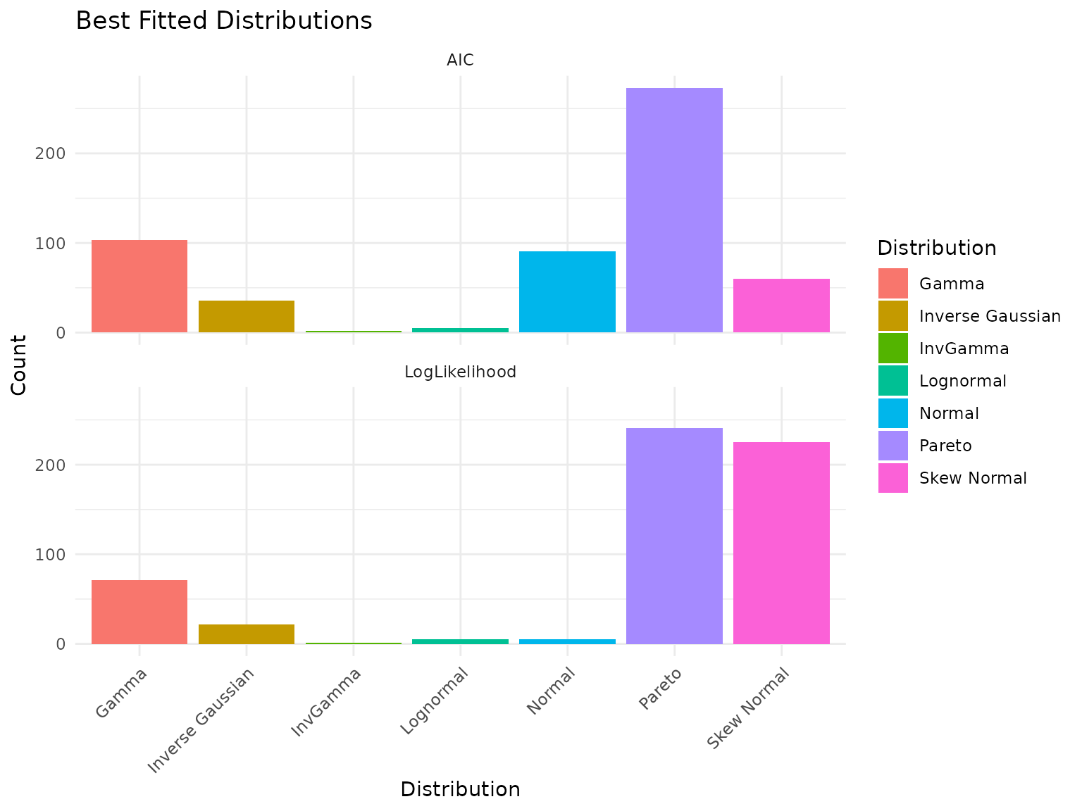
Best-fit distribution counts for PRM data.
Interpreting Distribution Fitting: A Cautionary Note
Important: Like the DDA dataset, we see that certain distributions may dominate the “best fit” counts. This is an artifact of small sample size (only 6 observations per peptide when averaged across tech reps), not a statement about true underlying distributions.
With more biological replicates, we would expect gamma and lognormal distributions to fit better - these are the typical distributions for mass spectrometry abundance data.
Parameter Distribution
p <- plot_param_distribution(fits)
print(p)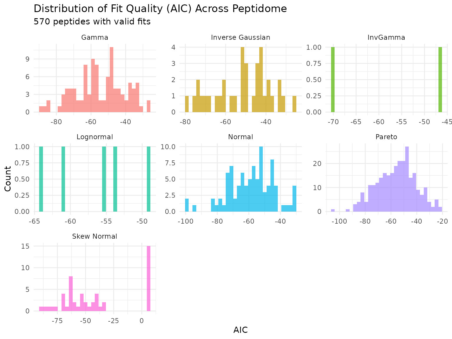
Distribution of AIC values across peptides for each fitted distribution.
# Count peptides per best-fit distribution
cat("\nPeptides per best-fit distribution:\n")
##
## Peptides per best-fit distribution:## # A tibble: 7 × 2
## distribution n
## <chr> <int>
## 1 Pareto 273
## 2 Gamma 103
## 3 Normal 91
## 4 Skew Normal 60
## 5 Inverse Gaussian 36
## 6 Lognormal 5
## 7 InvGamma 2Power Analysis
Choosing the Right Statistical Test
Critical first step: With small samples (N=3), test choice dramatically affects power. Before committing to detailed analyses, we compare available tests.
| Test | Type | Characteristics |
|---|---|---|
| Wilcoxon rank-sum | Non-parametric | Conservative, robust to outliers, needs larger N |
| Bootstrap-t | Resampling | Handles non-normality through resampling |
| Bayes factor | Bayesian | Evidence-based, often more powerful at small N |
# Run all three tests (use n_sim = 100 for faster rendering)
power_wilcox <- power_analysis(fits, effect_size = 2, n_per_group = 3,
                                find = "power", test = "wilcoxon", n_sim = 100)

power_boot <- power_analysis(fits, effect_size = 2, n_per_group = 3,
                              find = "power", test = "bootstrap_t", n_sim = 100)

power_bayes <- power_analysis(fits, effect_size = 2, n_per_group = 3,
                               find = "power", test = "bayes_t", n_sim = 100)

# Create comparison table
comparison <- tibble(
  Test = c("Wilcoxon rank-sum", "Bootstrap-t", "Bayes factor"),
  `Median Power` = c(
    median(power_wilcox$simulations$peptide_power, na.rm = TRUE),
    median(power_boot$simulations$peptide_power, na.rm = TRUE),
    median(power_bayes$simulations$peptide_power, na.rm = TRUE)
  ),
  `% > 50% Power` = c(
    mean(power_wilcox$simulations$peptide_power > 0.5, na.rm = TRUE) * 100,
    mean(power_boot$simulations$peptide_power > 0.5, na.rm = TRUE) * 100,
    mean(power_bayes$simulations$peptide_power > 0.5, na.rm = TRUE) * 100
  ),
  `% > 80% Power` = c(
    mean(power_wilcox$simulations$peptide_power > 0.8, na.rm = TRUE) * 100,
    mean(power_boot$simulations$peptide_power > 0.8, na.rm = TRUE) * 100,
    mean(power_bayes$simulations$peptide_power > 0.8, na.rm = TRUE) * 100
  )
)

knitr::kable(comparison, digits = 2,
caption = "Power comparison across statistical tests (N=3, 2-fold effect)")| Test | Median Power | % > 50% Power | % > 80% Power |
|---|---|---|---|
| Wilcoxon rank-sum | 0.00 | 0.00 | 0.00 |
| Bootstrap-t | 0.20 | 9.85 | 4.74 |
| Bayes factor | 0.56 | 64.60 | 16.06 |
Understanding the Test Comparison Results
The table above shows how different tests perform at small sample sizes:
Wilcoxon rank-sum is conservative - non-parametric tests trade statistical assumptions for larger sample size requirements.
Bootstrap-t uses resampling to handle non-normality, potentially offering intermediate power.
Bayes factor tests quantify evidence for an effect, often performing better at small N.
For remaining analyses: We use the Bayes factor test since it provides usable power estimates at N=3.
The Three Questions
Power analysis can answer three related questions:
- Power: Given N and effect size, what power do we have?
- Sample size: Given target power and effect size, what N do we need?
- Minimum detectable effect: Given N and target power, what effect can we detect?
Question 1: What Power Do We Have?
With 3 biological replicates and a 2-fold effect, what power do we achieve?
# Using Bayes factor test based on comparison results
power_current <- power_analysis(fits, effect_size = 2, n_per_group = 3,
                                 find = "power", test = "bayes_t", n_sim = 100)
print(power_current)
## peppwr_power analysis
## ---------------------
## Mode: per_peptide
##
## Power: 60%
## Sample size: 3 per group
## Effect size: 2.00-fold
##
## Statistical test: bayes_t
## Decision threshold: BF > 3 (substantial evidence)
plot(power_current)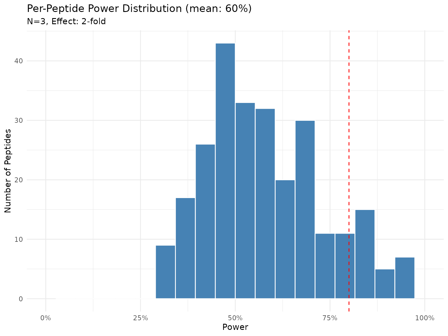
Distribution of power across peptides with N=3 and 2-fold effect (Bayes factor test).
Question 2: What Sample Size Do We Need?
What N would achieve 80% power to detect a 2-fold change?
sample_size <- power_analysis(fits, effect_size = 2, target_power = 0.8,
                              find = "sample_size", test = "bayes_t", n_sim = 100)
print(sample_size)
## peppwr_power analysis
## ---------------------
## Mode: per_peptide
##
## Recommended sample size: N=10 per group
## Target power: 80%
## Effect size: 2.00-fold
##
## Statistical test: bayes_t
## Decision threshold: BF > 3 (substantial evidence)
plot(sample_size)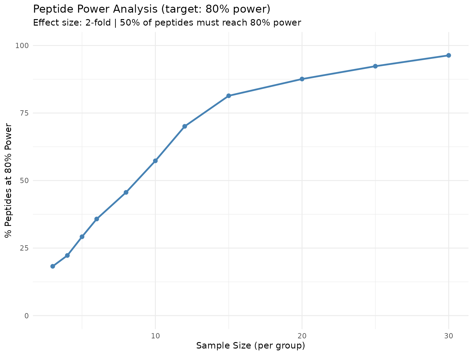
Percentage of peptides achieving 80% power at each sample size.
Question 3: What’s the Minimum Detectable Effect?
At N=3, what’s the smallest effect we can reliably detect?
Understanding the two thresholds: In per-peptide mode, there are two distinct thresholds:
-
target_power(set to 0.8) - The power level each individual peptide must achieve -
proportion_threshold(default 0.5) - The fraction of peptides that must reachtarget_power
The plot shows “% of peptides reaching 80% power” on the y-axis. The answer tells us: “At what effect size do 50% of peptides achieve 80% power?”
min_effect <- power_analysis(fits, n_per_group = 3, target_power = 0.8,
                             find = "effect_size", test = "bayes_t", n_sim = 100)
print(min_effect)
## peppwr_power analysis
## ---------------------
## Mode: per_peptide
##
## Minimum detectable effect: 5.00-fold
## Sample size: 3 per group
## Target power: 80%
##
## Statistical test: bayes_t
## Decision threshold: BF > 3 (substantial evidence)
plot(min_effect)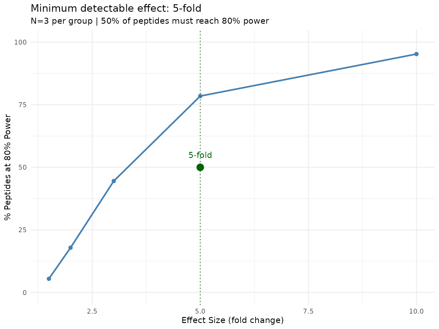
Proportion of peptides reaching 80% power at each effect size. The default threshold is 50% of peptides.
This tells us what effect sizes are realistically detectable with
current sample sizes. To require more peptides to be well-powered,
increase proportion_threshold.
Impact of Missingness on Power
How does accounting for missingness affect power estimates?
# Power without accounting for missingness (optimistic)
power_no_miss <- power_analysis(fits, effect_size = 2, n_per_group = 3,
                                 find = "power", test = "bayes_t",
                                 include_missingness = FALSE, n_sim = 100)

# Power accounting for missingness (realistic)
power_with_miss <- power_analysis(fits, effect_size = 2, n_per_group = 3,
                                   find = "power", test = "bayes_t",
                                   include_missingness = TRUE, n_sim = 100)

cat("Median power WITHOUT missingness:",
    round(median(power_no_miss$simulations$peptide_power, na.rm = TRUE), 3), "\n")
## Median power WITHOUT missingness: 0.575
cat("Median power WITH missingness:   ",
    round(median(power_with_miss$simulations$peptide_power, na.rm = TRUE), 3), "\n")
## Median power WITH missingness: 0.565Accounting for missingness typically reduces power estimates - this is the realistic cost of missing data on your experiment’s ability to detect effects.
FDR-Aware Power Analysis
Why FDR Matters
With 285 peptides tested, multiple testing is a concern. If we use alpha = 0.05 for each test, we expect ~14 false positives by chance alone (285 x 0.05 = 14.25).
FDR (False Discovery Rate) control methods like Benjamini-Hochberg adjust p-values to control the expected proportion of false discoveries. This is more stringent than nominal testing and reduces power.
Understanding prop_null
The prop_null parameter specifies the assumed proportion
of true null hypotheses - peptides with no real effect. This affects FDR
correction stringency:
prop_null |
Meaning | Impact |
|---|---|---|
| 0.9 | 90% of peptides have no effect | More stringent correction |
| 0.5 | 50% have real effects | Less stringent correction |
In targeted proteomics, you typically select peptides expected to
change, so prop_null might be lower than in discovery
experiments.
Standard vs FDR-Corrected Power
Note: FDR-aware mode requires frequentist tests (Wilcoxon or bootstrap-t) because Benjamini-Hochberg correction operates on p-values. Bayes factors cannot be meaningfully converted to p-values for this correction.
# Standard power with Wilcoxon (nominal alpha = 0.05)
power_nominal <- power_analysis(fits, effect_size = 2, n_per_group = 3,
                                find = "power", test = "wilcoxon",
                                apply_fdr = FALSE, n_sim = 100)

# FDR-aware power (BH correction)
# prop_null = 0.8 means we assume 80% of peptides have no true effect
power_fdr <- power_analysis(fits, effect_size = 2, n_per_group = 3,
                            find = "power", test = "wilcoxon",
                            apply_fdr = TRUE, prop_null = 0.8,
                            fdr_threshold = 0.05, n_sim = 100)
# Extract power values safely
nominal_power <- power_nominal$simulations$peptide_power
fdr_power <- power_fdr$simulations$peptide_power

cat("Nominal power (Wilcoxon, no FDR correction):\n")
## Nominal power (Wilcoxon, no FDR correction):
if (is.numeric(nominal_power) && length(nominal_power) > 0) {
  cat("  Median power:", round(median(nominal_power, na.rm = TRUE), 3), "\n")
  cat("  % peptides > 80% power:", round(mean(nominal_power > 0.8, na.rm = TRUE) * 100, 1), "%\n")
} else {
  print(power_nominal)
}
## Median power: 0
## % peptides > 80% power: 0 %
cat("\nFDR-aware power (Wilcoxon, BH correction, 80% true nulls):\n")##
## FDR-aware power (Wilcoxon, BH correction, 80% true nulls):
if (is.numeric(fdr_power) && length(fdr_power) > 0) {
  cat("  Median power:", round(median(fdr_power, na.rm = TRUE), 3), "\n")
  cat("  % peptides > 80% power:", round(mean(fdr_power > 0.8, na.rm = TRUE) * 100, 1), "%\n")
} else {
  print(power_fdr)
}
## peppwr_power analysis
## ---------------------
## Mode: per_peptide
##
## Power: 0%
## Sample size: 3 per group
## Effect size: 2.00-fold
##
## Statistical test: wilcoxon
## Significance level: 0.05
##
## FDR-adjusted analysis (Benjamini-Hochberg)
## Proportion true nulls: 80%
## FDR threshold: 5%Understanding the FDR Impact
FDR correction reduces power because:
- More evidence required: Adjusted p-values are larger, requiring stronger effects to reach significance
- Depends on number of tests: More peptides = more stringent correction
-
Depends on true effect proportion: If most peptides
have true effects (
prop_nullis low), FDR correction is less severe
For a targeted panel of 285 peptides, the FDR impact is more modest than for discovery proteomics with thousands of tests.
Summary and Recommendations
Key Findings
Missingness patterns: This PRM dataset has ~17% missing values. Some peptides may show evidence of MNAR (informative missingness), where low-abundance values are preferentially missing.
Distribution fitting: With only 6 observations per peptide (after averaging tech reps), distribution selection is unreliable. This is a small sample size artifact, not a reflection of true underlying distributions.
Test selection: Different statistical tests show varying power at small N. Bayes factor tests can provide more informative estimates than conservative non-parametric tests when samples are limited.
Missingness impact: Accounting for missing data reduces power estimates - this reflects the real cost of missingness.
FDR impact: With 285 peptides, FDR correction modestly reduces power compared to nominal testing.
Practical Recommendations
For future experiments: Consider N=6 or more biological replicates for reliable detection of 2-fold changes.
For current data: Set realistic expectations about detectable effect sizes. Subtle changes may not be detectable with N=3.
Test selection: With small samples, Bayes factor tests may be more informative than traditional frequentist approaches.
MNAR patterns: If dataset-level MNAR is detected, low-abundance peptide results should be interpreted cautiously.
Caveats
- This analysis combines both genotypes; genotype-specific analyses may differ
- Technical replicate averaging reduces noise but masks technical variability
- MNAR models are approximations; true missing data mechanisms may be more complex
- The
prop_nullparameter requires assumptions about true effect rates - Distribution fitting is limited by small sample size
Session Info
## R version 4.5.3 (2026-03-11)
## Platform: x86_64-pc-linux-gnu
## Running under: Ubuntu 24.04.4 LTS
##
## Matrix products: default
## BLAS:   /usr/lib/x86_64-linux-gnu/openblas-pthread/libblas.so.3
## LAPACK: /usr/lib/x86_64-linux-gnu/openblas-pthread/libopenblasp-r0.3.26.so;  LAPACK version 3.12.0
##
## locale:
##  [1] LC_CTYPE=C.UTF-8       LC_NUMERIC=C           LC_TIME=C.UTF-8
##  [4] LC_COLLATE=C.UTF-8     LC_MONETARY=C.UTF-8    LC_MESSAGES=C.UTF-8
##  [7] LC_PAPER=C.UTF-8       LC_NAME=C              LC_ADDRESS=C
## [10] LC_TELEPHONE=C         LC_MEASUREMENT=C.UTF-8 LC_IDENTIFICATION=C
##
## time zone: UTC
## tzcode source: system (glibc)
##
## attached base packages:
## [1] stats     graphics  grDevices datasets  utils     methods   base
##
## other attached packages:
## [1] tibble_3.3.1  ggplot2_4.0.2 dplyr_1.2.1   peppwR_0.1.0
##
## loaded via a namespace (and not attached):
##  [1] sass_0.4.10         utf8_1.2.6          generics_0.1.4
##  [4] tidyr_1.3.2         renv_0.12.2         lattice_0.22-9
##  [7] fGarch_4052.93      digest_0.6.39       magrittr_2.0.5
## [10] evaluate_1.0.5      grid_4.5.3          RColorBrewer_1.1-3
## [13] fastmap_1.2.0       Matrix_1.7-4        jsonlite_2.0.0
## [16] mgcv_1.9-4          purrr_1.2.2         scales_1.4.0
## [19] gbutils_0.5.1       textshaping_1.0.5   jquerylib_0.1.4
## [22] Rdpack_2.6.6        cli_3.6.6           timeSeries_4052.112
## [25] rlang_1.2.0         rbibutils_2.4.1     splines_4.5.3
## [28] cowplot_1.2.0       intervals_0.15.5    withr_3.0.2
## [31] cachem_1.1.0        yaml_2.3.12         cvar_0.6
## [34] tools_4.5.3         assertthat_0.2.1    vctrs_0.7.3
## [37] R6_2.6.1            lifecycle_1.0.5     fs_2.0.1
## [40] univariateML_1.5.0  ragg_1.5.2          pkgconfig_2.0.3
## [43] desc_1.4.3          pkgdown_2.2.0       pillar_1.11.1
## [46] bslib_0.10.0        gtable_0.3.6        glue_1.8.0
## [49] systemfonts_1.3.2   xfun_0.57           tidyselect_1.2.1
## [52] knitr_1.51          farver_2.1.2        spatial_7.3-18
## [55] nlme_3.1-168        htmltools_0.5.9     fBasics_4052.98
## [58] labeling_0.4.3      rmarkdown_2.31      timeDate_4052.112
## [61] compiler_4.5.3      S7_0.2.1-1