Power Analysis for Time-Course Phosphoproteomics (DDA)

Introduction

What is Statistical Power?

Statistical power is the probability of detecting a true effect when one exists. In proteomics experiments, this translates to: “If a phosphopeptide truly changes between conditions, how likely are we to find it statistically significant?”

Power depends on four interconnected factors:

Effect size - How large is the biological change? (e.g., 2-fold)
Sample size - How many biological replicates per group?
Variability - How noisy is the measurement?
Significance threshold - What alpha level are we using? (typically 0.05)

Why Does Power Matter?

Phosphoproteomics experiments are expensive and time-consuming. Under-powered experiments waste resources by failing to detect real biological changes. Over-powered experiments waste resources by using more samples than necessary.

Power analysis helps researchers:

Before an experiment: Determine required sample size for adequate power
After a pilot: Assess what effects can be detected with current data
For grant planning: Justify sample size requirements to reviewers

The peppwR Approach

peppwR uses simulation-based power analysis:

Fit distributions to pilot data to capture realistic abundance patterns
Simulate experiments by drawing from fitted distributions
Apply statistical tests to simulated data
Estimate power as the proportion of simulations with significant results

This approach captures the full complexity of phosphoproteomics data, including heterogeneity across peptides.

About the Data

This analysis uses Arabidopsis phosphoproteomics data from a time-course experiment:

Property	Value
Method	DDA (Data-Dependent Acquisition) mass spectrometry
Comparison	Early (t=0) vs late (t=600) timepoints
Biological replicates	3 per condition
Total observations per peptide	6 (important limitation!)
Peptides	2,228 phosphopeptides quantified
Missing data	None (complete observations)

Data Preparation

library(peppwR)
library(dplyr)
library(ggplot2)
library(tibble)

# Load the DDA experiment data
dda <- read.csv("../../sample_data/dda_data.csv")

# Examine the structure
glimpse(dda)

## Rows: 26,820
## Columns: 7
## $ protein_name      <chr> "PROT_0001", "PROT_0001", "PROT_0001", "PROT_0001", …
## $ genotype          <chr> "Genotype_A", "Genotype_A", "Genotype_A", "Genotype_…
## $ bio_rep           <int> 1, 2, 3, 1, 2, 3, 1, 2, 3, 1, 2, 3, 1, 2, 3, 1, 2, 3…
## $ tech_rep          <int> 0, 0, 0, 0, 0, 0, 0, 0, 0, 0, 0, 0, 0, 0, 0, 0, 0, 0…
## $ timepoints        <int> 0, 0, 0, 150, 150, 150, 300, 300, 300, 600, 600, 600…
## $ timepoints_values <dbl> 111486.89, 169993.66, 7241966.48, 174394.39, 2955899…
## $ new_annotation    <chr> "PEP_00001", "PEP_00001", "PEP_00001", "PEP_00001", …

# Filter to early (0) vs late (600) timepoints and format for peppwR
pilot <- dda |>
  filter(timepoints %in% c(0, 600)) |>
  transmute(
    peptide_id = new_annotation,
    condition = paste0("t", timepoints),
    abundance = timepoints_values
  )

# Summary statistics
cat("Unique peptides:", n_distinct(pilot$peptide_id), "\n")

## Unique peptides: 2228

cat("Observations per condition:\n")

## Observations per condition:

pilot |> count(condition)

##   condition    n
## 1        t0 6705
## 2      t600 6705

# Exploratory visualization
ggplot(pilot, aes(x = log2(abundance), fill = condition)) +
  geom_density(alpha = 0.5) +
  labs(
    x = "Log2 Abundance",
    y = "Density",
    title = "Phosphopeptide Abundance Distribution"
  ) +
  theme_minimal()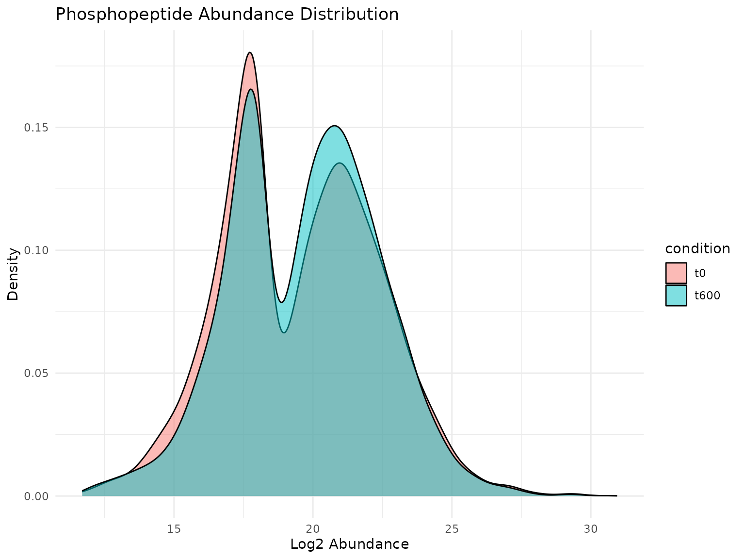

Distribution of log2 abundance values across conditions. The broad range and right-skew are typical for phosphoproteomics data.

The abundance values span several orders of magnitude, typical for phosphoproteomics data. The distributions appear similar between timepoints at the global level, though individual peptides may show significant changes.

Distribution Fitting

Why Fit Distributions?

To simulate realistic experiments, we need parametric models that capture the statistical properties of each peptide’s abundance values. peppwR fits multiple candidate distributions (gamma, lognormal, inverse Gaussian, Pareto, skew normal, etc.) and selects the best fit for each peptide based on AIC.

# Fit distributions to each peptide
fits <- fit_distributions(pilot, "peptide_id", "condition", "abundance")

# Summary of fitting results
print(fits)

## peppwr_fits object
## ------------------
## 4456 peptides fitted
## 
## Best fit distribution counts:
##   Gamma: 416
##   Inverse Gaussian: 1
##   Loggamma: 1
##   Normal: 515
##   Pareto: 3522
##   Skew Normal: 1

# Visualize which distributions fit best
plot(fits)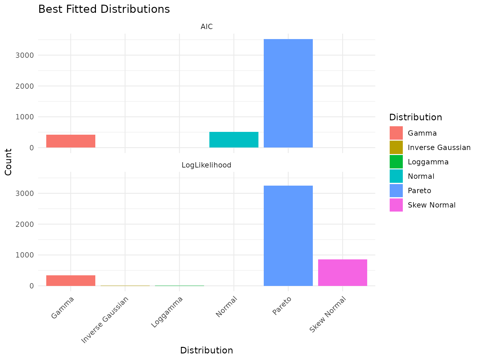

Best-fit distribution counts across the peptidome.

Interpreting Distribution Fitting Results: A Cautionary Note

Important: With only 6 observations per peptide (3 replicates x 2 conditions), distribution selection is unreliable. You may observe that distributions like Pareto or Skew Normal dominate the “best fit” counts. This is an artifact of small sample size, not a statement about the true underlying distributions.

With more biological replicates, we would expect gamma and lognormal distributions to fit better - these are the typical distributions for mass spectrometry abundance data based on the underlying measurement process.

Key insight: The specific distribution matters less than having enough data to fit it reliably. For power analysis, we proceed with the best available fits while acknowledging this limitation.

Parameter Distribution

p <- plot_param_distribution(fits)
print(p)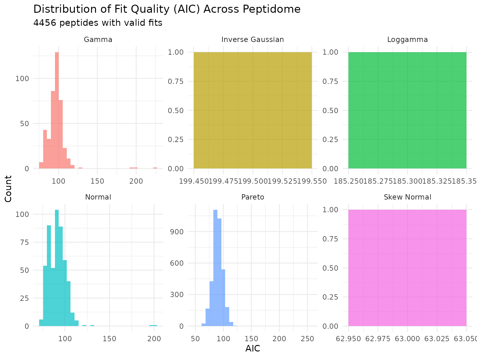

Distribution of AIC values across peptides for each fitted distribution. Lower AIC indicates better fit.

# Count peptides per best-fit distribution for context
cat("\nPeptides per best-fit distribution:\n")

## 
## Peptides per best-fit distribution:

tibble(distribution = fits$best) |>
  count(distribution) |>
  arrange(desc(n))

## # A tibble: 6 × 2
##   distribution         n
##   <chr>            <int>
## 1 Pareto            3522
## 2 Normal             515
## 3 Gamma              416
## 4 Inverse Gaussian     1
## 5 Loggamma             1
## 6 Skew Normal          1

Power Analysis

Choosing the Right Statistical Test

Critical first step: With small samples (N=3), the choice of statistical test dramatically affects power. Before proceeding with detailed analysis, we must compare tests to understand their behavior.

peppwR supports several tests:

Test	Type	Characteristics
Wilcoxon rank-sum	Non-parametric	Conservative, robust to outliers, needs larger N
Bootstrap-t	Resampling	Handles non-normality through resampling
Bayes factor	Bayesian	Evidence-based, often more powerful at small N

Let’s compare all three tests at N=3 with a 2-fold effect:

# Run all three tests (use n_sim = 100 for faster rendering)
power_wilcox <- power_analysis(fits, effect_size = 2, n_per_group = 3,
                                find = "power", test = "wilcoxon", n_sim = 100)

power_boot <- power_analysis(fits, effect_size = 2, n_per_group = 3,
                              find = "power", test = "bootstrap_t", n_sim = 100)

power_bayes <- power_analysis(fits, effect_size = 2, n_per_group = 3,
                               find = "power", test = "bayes_t", n_sim = 100)

# Create comparison table
comparison <- tibble(
  Test = c("Wilcoxon rank-sum", "Bootstrap-t", "Bayes factor"),
  `Median Power` = c(
    median(power_wilcox$simulations$peptide_power, na.rm = TRUE),
    median(power_boot$simulations$peptide_power, na.rm = TRUE),
    median(power_bayes$simulations$peptide_power, na.rm = TRUE)
  ),
  `% > 50% Power` = c(
    mean(power_wilcox$simulations$peptide_power > 0.5, na.rm = TRUE) * 100,
    mean(power_boot$simulations$peptide_power > 0.5, na.rm = TRUE) * 100,
    mean(power_bayes$simulations$peptide_power > 0.5, na.rm = TRUE) * 100
  ),
  `% > 80% Power` = c(
    mean(power_wilcox$simulations$peptide_power > 0.8, na.rm = TRUE) * 100,
    mean(power_boot$simulations$peptide_power > 0.8, na.rm = TRUE) * 100,
    mean(power_bayes$simulations$peptide_power > 0.8, na.rm = TRUE) * 100
  )
)

knitr::kable(comparison, digits = 2,
             caption = "Power comparison across statistical tests (N=3, 2-fold effect)")

Power comparison across statistical tests (N=3, 2-fold effect)
Test	Median Power	% > 50% Power	% > 80% Power
Wilcoxon rank-sum	0.00	0.00	0.00
Bootstrap-t	0.15	2.68	0.11
Bayes factor	0.47	40.73	5.79

Understanding the Test Comparison Results

The comparison table reveals important insights:

Wilcoxon rank-sum is conservative with small samples. Non-parametric tests don’t make distributional assumptions, but this comes at a cost: they need more data to achieve comparable power.
Bootstrap-t uses resampling to handle non-normality, potentially offering better power than Wilcoxon.
Bayes factor tests provide evidence for or against an effect. At small N, Bayesian approaches can be more informative than frequentist tests.

Recommendation: For the remaining analyses in this document, we use the Bayes factor test since it provides usable power estimates at N=3.

The Three Questions

Power analysis can answer three related questions about experimental design:

Power: Given sample size and effect size, what is my power?
Sample size: Given target power and effect size, what N do I need?
Minimum detectable effect: Given sample size and target power, what’s the smallest effect I can detect?

These questions are mathematically related - fixing any three parameters determines the fourth.

Question 1: Current Power (N=3)

With 3 biological replicates per group (as in this experiment), what power do we have to detect a 2-fold change?

# Using Bayes factor test based on our comparison results
power_n3 <- power_analysis(fits, effect_size = 2, n_per_group = 3,
                           find = "power", test = "bayes_t", n_sim = 100)
print(power_n3)

## peppwr_power analysis
## ---------------------
## Mode: per_peptide
## 
## Power: 51%
## Sample size: 3 per group
## Effect size: 2.00-fold
## 
## Statistical test: bayes_t
## Decision threshold: BF > 3 (substantial evidence)

plot(power_n3)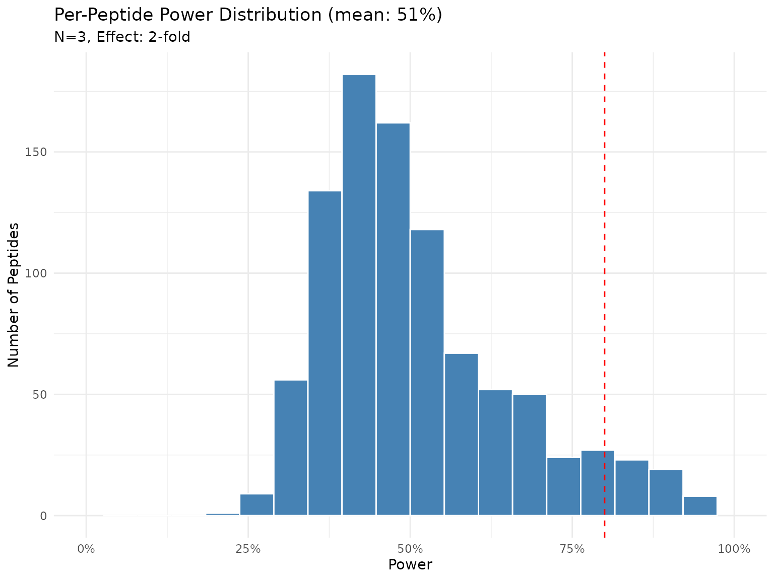

Distribution of power across peptides with N=3 and 2-fold effect (Bayes factor test). Each bar represents the proportion of peptides achieving that power level.

With N=3, power to detect a 2-fold change varies across peptides. Peptides with lower variability will have higher power, while noisy peptides remain under-powered.

Question 2: Sample Size for Target Power

What sample size would we need to achieve 80% power to detect a 2-fold change for most peptides?

sample_size <- power_analysis(fits, effect_size = 2, target_power = 0.8,
                              find = "sample_size", test = "bayes_t", n_sim = 100)
print(sample_size)

## peppwr_power analysis
## ---------------------
## Mode: per_peptide
## 
## Recommended sample size: N=15 per group
## Target power: 80%
## Effect size: 2.00-fold
## 
## Statistical test: bayes_t
## Decision threshold: BF > 3 (substantial evidence)

plot(sample_size)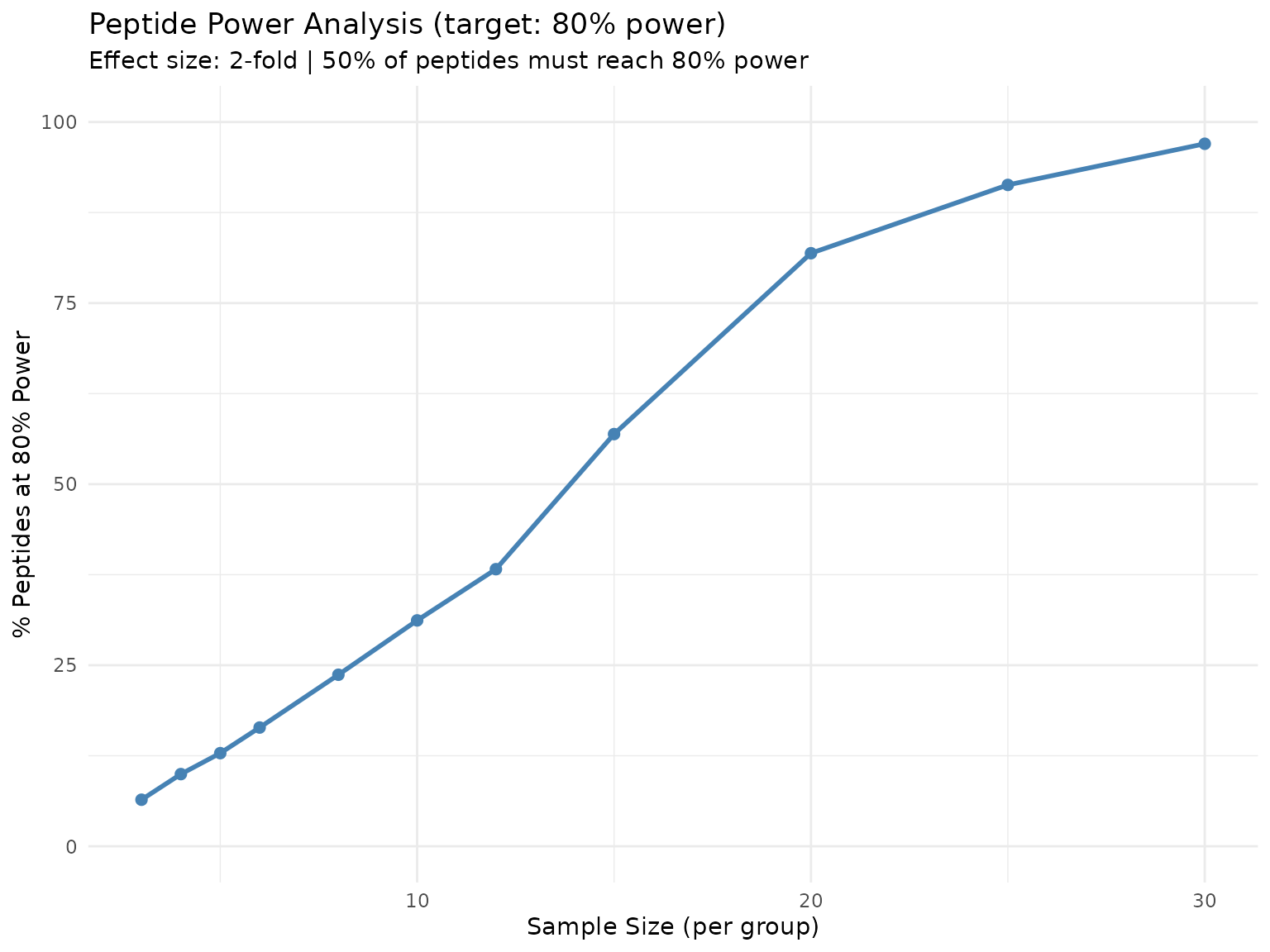

Percentage of peptides reaching 80% power at each sample size. The curve shows diminishing returns as N increases.

This curve directly answers “what percentage of my peptides will be well-powered at sample size N?” - useful for experimental planning when budget constraints limit replication.

Question 3: Minimum Detectable Effect

At N=3 with 80% power target, what’s the smallest effect we can reliably detect?

Understanding the two thresholds: In per-peptide mode, there are two distinct thresholds:

target_power (set to 0.8) - The power level each individual peptide must achieve
proportion_threshold (default 0.5) - The fraction of peptides that must reach target_power

The plot shows “% of peptides reaching 80% power” on the y-axis. The answer tells us: “At what effect size do 50% of peptides achieve 80% power?”

min_effect <- power_analysis(fits, n_per_group = 3, target_power = 0.8,
                             find = "effect_size", test = "bayes_t", n_sim = 100)
print(min_effect)

## peppwr_power analysis
## ---------------------
## Mode: per_peptide
## 
## Minimum detectable effect: 10.00-fold
## Sample size: 3 per group
## Target power: 80%
## 
## Statistical test: bayes_t
## Decision threshold: BF > 3 (substantial evidence)

plot(min_effect)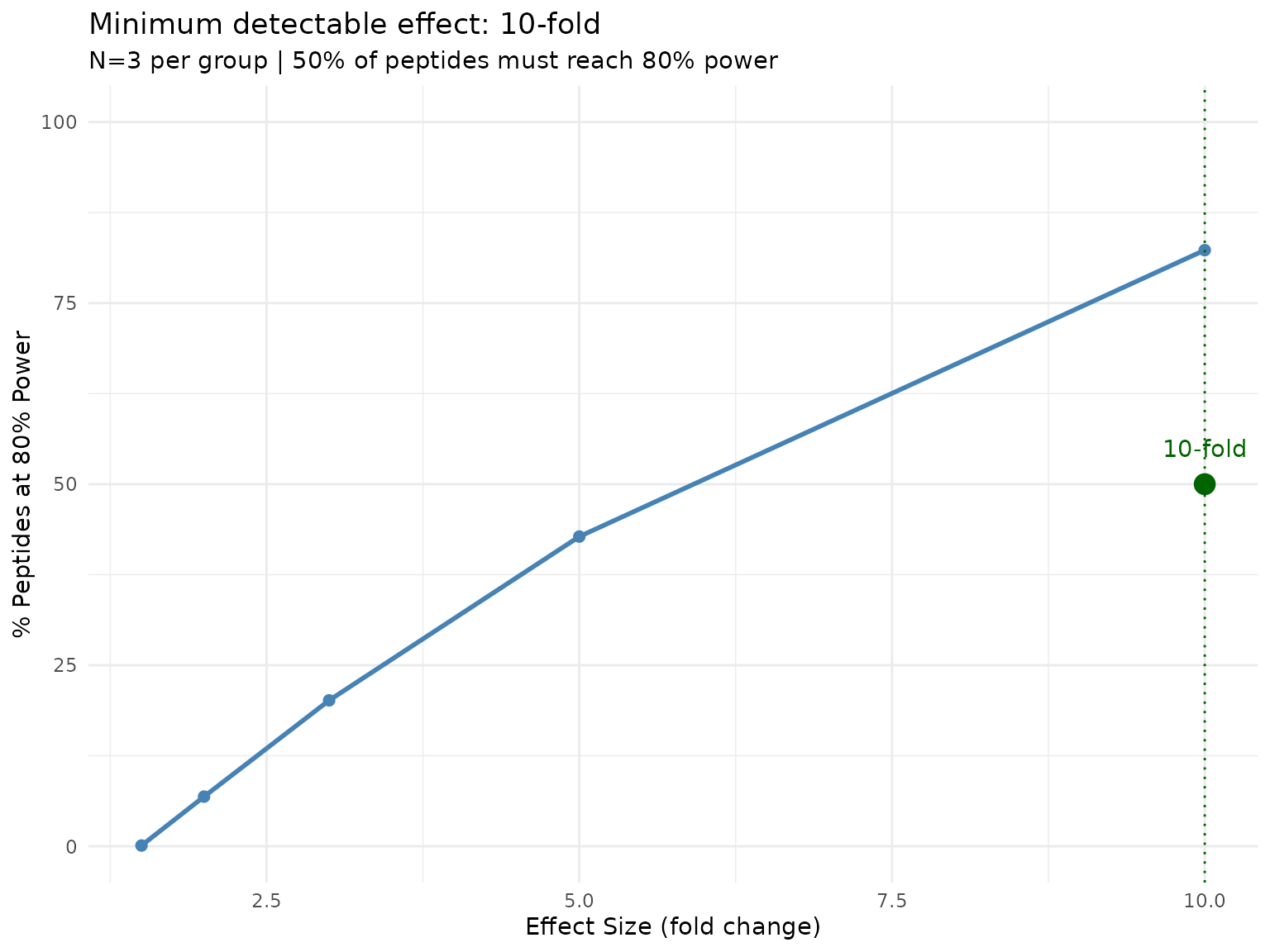

Proportion of peptides reaching 80% power at each effect size. The default threshold is 50% of peptides (proportion_threshold = 0.5).

With only N=3, very large effects are needed for a majority of peptides to be well-powered. This is a realistic but sobering assessment of what under-powered experiments can detect.

To require a higher fraction of peptides to be well-powered, increase proportion_threshold:

# Require 80% of peptides to reach 80% power (stricter)
power_analysis(fits, n_per_group = 3, target_power = 0.8,
               find = "effect_size", proportion_threshold = 0.8, ...)

Power Heatmap

A power heatmap visualizes how power varies across combinations of sample size and effect size - useful for identifying the “sweet spot” for experimental design.

Why Aggregate Mode for Heatmaps?

The plot_power_heatmap() function uses aggregate mode (single distribution) rather than per-peptide mode because:

Computational cost: Per-peptide heatmaps would require millions of simulations
Visualization: A single heatmap is more interpretable than 2000+ individual heatmaps
Purpose: Heatmaps answer “what’s the general tradeoff?” not “what’s the power for peptide X?”

To make the heatmap relevant to your data, we derive representative parameters from the fitted distributions:

# Derive representative parameters from the data
log_abundances <- log(pilot$abundance[pilot$abundance > 0])
derived_params <- list(
  meanlog = median(log_abundances),
  sdlog = mad(log_abundances, constant = 1)  # robust SD estimate
)

cat("Using representative lognormal parameters:\n")

## Using representative lognormal parameters:

cat("  meanlog =", round(derived_params$meanlog, 2), "\n")

##   meanlog = 13.72

cat("  sdlog =", round(derived_params$sdlog, 2), "\n")

##   sdlog = 1.41

# Generate heatmap with data-derived parameters
plot_power_heatmap(
  distribution = "lnorm",
  params = derived_params,
  n_range = c(3, 12),
  effect_range = c(1.2, 3),
  test = "wilcoxon"  # heatmap uses aggregate mode
)

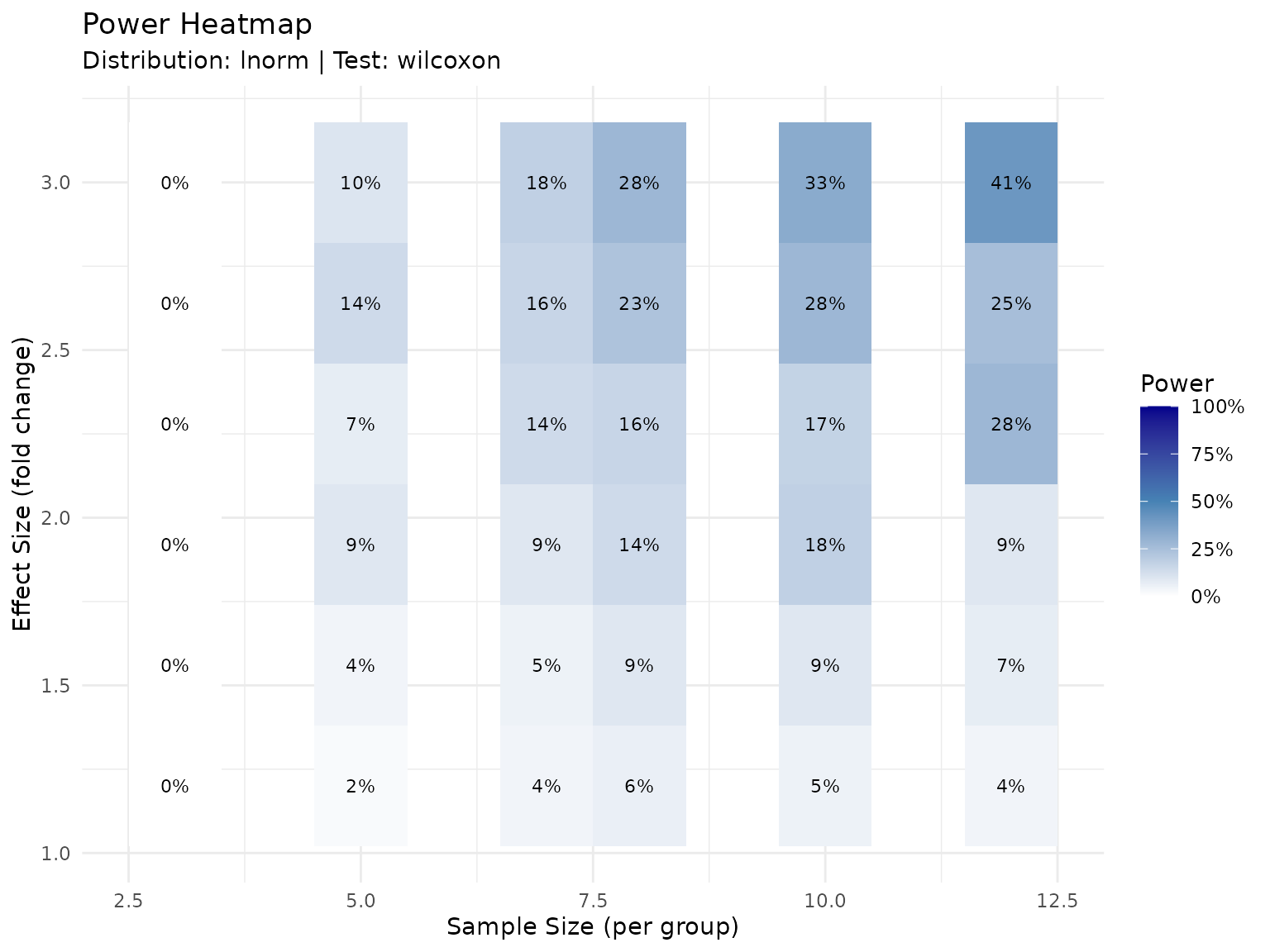
Power as a function of sample size and effect size for a representative peptide. Colors indicate expected power. Individual peptides will vary based on their specific variability.

Interpreting the Heatmap

The heatmap shows power for a representative peptide with typical abundance characteristics. Individual peptides will vary:

Low-variability peptides will have higher power than shown
High-variability peptides will have lower power than shown
Use the per-peptide find = "power" results to understand the distribution across peptides

The heatmap shows:

Lower-left corner (small N, small effect): Low power - avoid this region
Upper-right corner (large N, large effect): High power but potentially wasteful
Diagonal transition zone: The practical planning region where tradeoffs matter

Summary and Recommendations

Key Findings

Distribution fitting: With only 6 observations per peptide, distribution selection is unreliable. The observed “best fit” distributions are artifacts of small sample size, not the true underlying distributions.
Test selection matters: Wilcoxon rank-sum may have limited power at N=3 due to its conservative nature. Bayes factor tests can provide more informative power estimates with small samples.
Current power (N=3): With 3 replicates and the Bayes factor test, power to detect a 2-fold change varies across peptides based on their individual variability.
Sample size requirements: Achieving consistently high power (80%+) across most peptides requires more than N=3 biological replicates.
Minimum detectable effect: At N=3, only relatively large fold changes can be reliably detected at 80% power for most peptides.

Practical Recommendations

For future experiments: Consider N=6 or more biological replicates if detecting smaller fold changes (<2-fold) is important.
For current data interpretation: Results showing non-significance may reflect insufficient power rather than absence of biological effect. Be cautious about concluding “no difference.”
Test selection: With small samples, consider Bayes factor tests which may be more informative than traditional frequentist tests.
Effect size expectations: Set realistic expectations - detecting subtle changes requires adequate replication.

Caveats

This analysis uses a single genotype (Col-0) and specific timepoint comparison (0 vs 600)
Distribution fitting is limited by small sample size (6 observations per peptide)
Power estimates assume fitted distributions accurately represent underlying biology
Technical variability (not modeled here) may further reduce effective power
Real experimental factors (batch effects, sample quality) are not captured

Session Info

sessionInfo()

## R version 4.5.2 (2025-10-31)
## Platform: x86_64-pc-linux-gnu
## Running under: Ubuntu 24.04.3 LTS
## 
## Matrix products: default
## BLAS:   /usr/lib/x86_64-linux-gnu/openblas-pthread/libblas.so.3 
## LAPACK: /usr/lib/x86_64-linux-gnu/openblas-pthread/libopenblasp-r0.3.26.so;  LAPACK version 3.12.0
## 
## locale:
##  [1] LC_CTYPE=C.UTF-8       LC_NUMERIC=C           LC_TIME=C.UTF-8       
##  [4] LC_COLLATE=C.UTF-8     LC_MONETARY=C.UTF-8    LC_MESSAGES=C.UTF-8   
##  [7] LC_PAPER=C.UTF-8       LC_NAME=C              LC_ADDRESS=C          
## [10] LC_TELEPHONE=C         LC_MEASUREMENT=C.UTF-8 LC_IDENTIFICATION=C   
## 
## time zone: UTC
## tzcode source: system (glibc)
## 
## attached base packages:
## [1] stats     graphics  grDevices datasets  utils     methods   base     
## 
## other attached packages:
## [1] tibble_3.3.1  ggplot2_4.0.2 dplyr_1.2.0   peppwR_0.1.0 
## 
## loaded via a namespace (and not attached):
##  [1] utf8_1.2.6          sass_0.4.10         generics_0.1.4     
##  [4] tidyr_1.3.2         renv_0.12.2         lattice_0.22-7     
##  [7] fGarch_4052.93      digest_0.6.39       magrittr_2.0.4     
## [10] evaluate_1.0.5      grid_4.5.2          RColorBrewer_1.1-3 
## [13] fastmap_1.2.0       Matrix_1.7-4        jsonlite_2.0.0     
## [16] purrr_1.2.1         scales_1.4.0        gbutils_0.5.1      
## [19] textshaping_1.0.4   jquerylib_0.1.4     Rdpack_2.6.6       
## [22] cli_3.6.5           timeSeries_4052.112 rlang_1.1.7        
## [25] rbibutils_2.4.1     intervals_0.15.5    withr_3.0.2        
## [28] cachem_1.1.0        yaml_2.3.12         cvar_0.6           
## [31] tools_4.5.2         assertthat_0.2.1    vctrs_0.7.1        
## [34] R6_2.6.1            lifecycle_1.0.5     fs_1.6.6           
## [37] univariateML_1.5.0  ragg_1.5.0          pkgconfig_2.0.3    
## [40] desc_1.4.3          pkgdown_2.2.0       pillar_1.11.1      
## [43] bslib_0.10.0        gtable_0.3.6        glue_1.8.0         
## [46] systemfonts_1.3.1   xfun_0.56           tidyselect_1.2.1   
## [49] knitr_1.51          farver_2.1.2        spatial_7.3-18     
## [52] htmltools_0.5.9     fBasics_4052.98     rmarkdown_2.30     
## [55] labeling_0.4.3      timeDate_4052.112   compiler_4.5.2     
## [58] S7_0.2.1

peppwR

2026-02-09