Introduction
Proteomics datasets often contain thousands to tens of thousands of peptides. This vignette characterizes peppwR’s performance characteristics to help you:
- Estimate runtime for your dataset size
- Choose appropriate
n_simvalues - Understand memory requirements
- Make informed trade-offs between precision and compute time
Experimental Setup
Test Data Generator
generate_test_data <- function(n_peptides, n_per_group = 4, seed = 42) {
  set.seed(seed)

  peptide_params <- tibble::tibble(
    peptide_id = paste0("pep_", sprintf("%05d", 1:n_peptides)),
    shape = runif(n_peptides, 1.5, 5),
    rate = runif(n_peptides, 0.01, 0.1)
  )

  peptide_params |>
    dplyr::rowwise() |>
    dplyr::mutate(
      data = list(tibble::tibble(
        condition = rep(c("control", "treatment"), each = n_per_group),
        replicate = rep(1:n_per_group, 2),
        abundance = rgamma(n_per_group * 2, shape = shape, rate = rate)
      ))
    ) |>
    dplyr::ungroup() |>
    dplyr::select(peptide_id, data) |>
    tidyr::unnest(data)
}
Test Configurations
# Peptide counts for scaling tests
peptide_counts <- c(100, 500, 1000, 2000)

# Simulation counts for power analysis
sim_counts <- c(500, 1000, 2000)
Note: For practical vignette build times, we use smaller dataset sizes than the full specification (which includes 5000, 10000, 20000 peptides). Scale estimates linearly for larger datasets.
Distribution Fitting Scaling
Benchmark Fitting
All benchmarks use distributions = "continuous" which
fits distributions appropriate for continuous abundance data (gamma,
lognormal, normal, etc.).
fit_results <- bench::mark(
  `100 peptides` = fit_distributions(fit_data$n100, "peptide_id", "condition", "abundance",
                                      distributions = "continuous"),
  `500 peptides` = fit_distributions(fit_data$n500, "peptide_id", "condition", "abundance",
                                      distributions = "continuous"),
  `1000 peptides` = fit_distributions(fit_data$n1000, "peptide_id", "condition", "abundance",
                                       distributions = "continuous"),
  `2000 peptides` = fit_distributions(fit_data$n2000, "peptide_id", "condition", "abundance",
                                       distributions = "continuous"),
  iterations = 1,
  check = FALSE,
  memory = TRUE
)
#> Loading required namespace: intervals

fit_results_df <- tibble::tibble(
  peptides = peptide_counts,
  time_s = as.numeric(fit_results$median),
  memory_mb = as.numeric(fit_results$mem_alloc) / 1024^2
)

fit_results_df$time_per_peptide_ms <- fit_results_df$time_s * 1000 / fit_results_df$peptides

knitr::kable(
  fit_results_df,
  col.names = c("Peptides", "Time (s)", "Memory (MB)", "Time/peptide (ms)"),
  digits = 2,
  caption = "Distribution fitting scaling"
)| Peptides | Time (s) | Memory (MB) | Time/peptide (ms) |
|---|---|---|---|
| 100 | 3.21 | 101.31 | 32.11 |
| 500 | 15.69 | 9.77 | 31.38 |
| 1000 | 31.21 | 19.53 | 31.21 |
| 2000 | 62.42 | 39.05 | 31.21 |
Fitting Scaling Plot
ggplot2::ggplot(fit_results_df, ggplot2::aes(x = peptides, y = time_s)) +
  ggplot2::geom_point(size = 3, color = "steelblue") +
  ggplot2::geom_line(color = "steelblue") +
  ggplot2::scale_x_log10() +
  ggplot2::scale_y_log10() +
  ggplot2::theme_minimal() +
  ggplot2::labs(
    x = "Number of Peptides (log scale)",
    y = "Time (seconds, log scale)",
    title = "Distribution Fitting: Time vs Dataset Size"
  )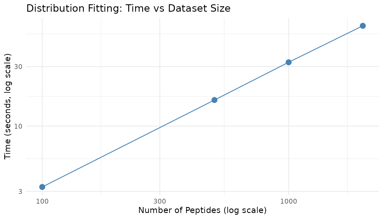
Distribution fitting scales approximately linearly with the number of peptides, as each peptide is fitted independently.
Power Analysis - Aggregate Mode
Aggregate mode performance depends primarily on n_sim,
not on any dataset size (since it simulates a single “typical”
peptide).
Effect of n_sim
set.seed(123)

agg_results <- bench::mark(
  `n_sim=500` = power_analysis("gamma", list(shape = 2, rate = 0.05),
                               effect_size = 2, n_per_group = 6,
                               find = "power", n_sim = 500),
  `n_sim=1000` = power_analysis("gamma", list(shape = 2, rate = 0.05),
                                effect_size = 2, n_per_group = 6,
                                find = "power", n_sim = 1000),
  `n_sim=2000` = power_analysis("gamma", list(shape = 2, rate = 0.05),
                                effect_size = 2, n_per_group = 6,
                                find = "power", n_sim = 2000),
  iterations = 3,
  check = FALSE
)

agg_df <- tibble::tibble(
  n_sim = sim_counts,
  time_s = as.numeric(agg_results$median)
)

knitr::kable(
  agg_df,
  col.names = c("n_sim", "Time (s)"),
  digits = 3,
  caption = "Aggregate mode timing by n_sim"
)| n_sim | Time (s) |
|---|---|
| 500 | 0.041 |
| 1000 | 0.082 |
| 2000 | 0.162 |
Power Estimate Stabilization
More simulations yield more stable power estimates. Let’s examine convergence:
set.seed(42)

# Run multiple times at each n_sim level
stabilization_data <- do.call(rbind, lapply(c(100, 250, 500, 1000, 2000), function(n) {
  powers <- replicate(10, {
    result <- power_analysis("gamma", list(shape = 2, rate = 0.05),
                            effect_size = 2, n_per_group = 6,
                            find = "power", n_sim = n)
    result$answer
  })

  tibble::tibble(
    n_sim = n,
    mean_power = mean(powers),
    sd_power = sd(powers),
    ci_width = 1.96 * sd(powers) * 2
  )
}))

knitr::kable(
  stabilization_data,
  col.names = c("n_sim", "Mean Power", "SD", "95% CI Width"),
  digits = 3,
  caption = "Power estimate stability by n_sim"
)| n_sim | Mean Power | SD | 95% CI Width |
|---|---|---|---|
| 100 | 0.267 | 0.063 | 0.246 |
| 250 | 0.255 | 0.032 | 0.127 |
| 500 | 0.255 | 0.020 | 0.078 |
| 1000 | 0.251 | 0.021 | 0.082 |
| 2000 | 0.254 | 0.008 | 0.033 |
ggplot2::ggplot(stabilization_data, ggplot2::aes(x = n_sim)) +
  ggplot2::geom_ribbon(
    ggplot2::aes(ymin = mean_power - 1.96 * sd_power,
                 ymax = mean_power + 1.96 * sd_power),
    fill = "steelblue", alpha = 0.3
  ) +
  ggplot2::geom_line(ggplot2::aes(y = mean_power), color = "steelblue", linewidth = 1) +
  ggplot2::geom_point(ggplot2::aes(y = mean_power), color = "steelblue", size = 2) +
  ggplot2::scale_x_log10() +
  ggplot2::theme_minimal() +
  ggplot2::labs(
    x = "Number of Simulations (log scale)",
    y = "Power Estimate",
    title = "Power Estimate Convergence",
    subtitle = "Shaded region shows 95% confidence interval across 10 runs"
  )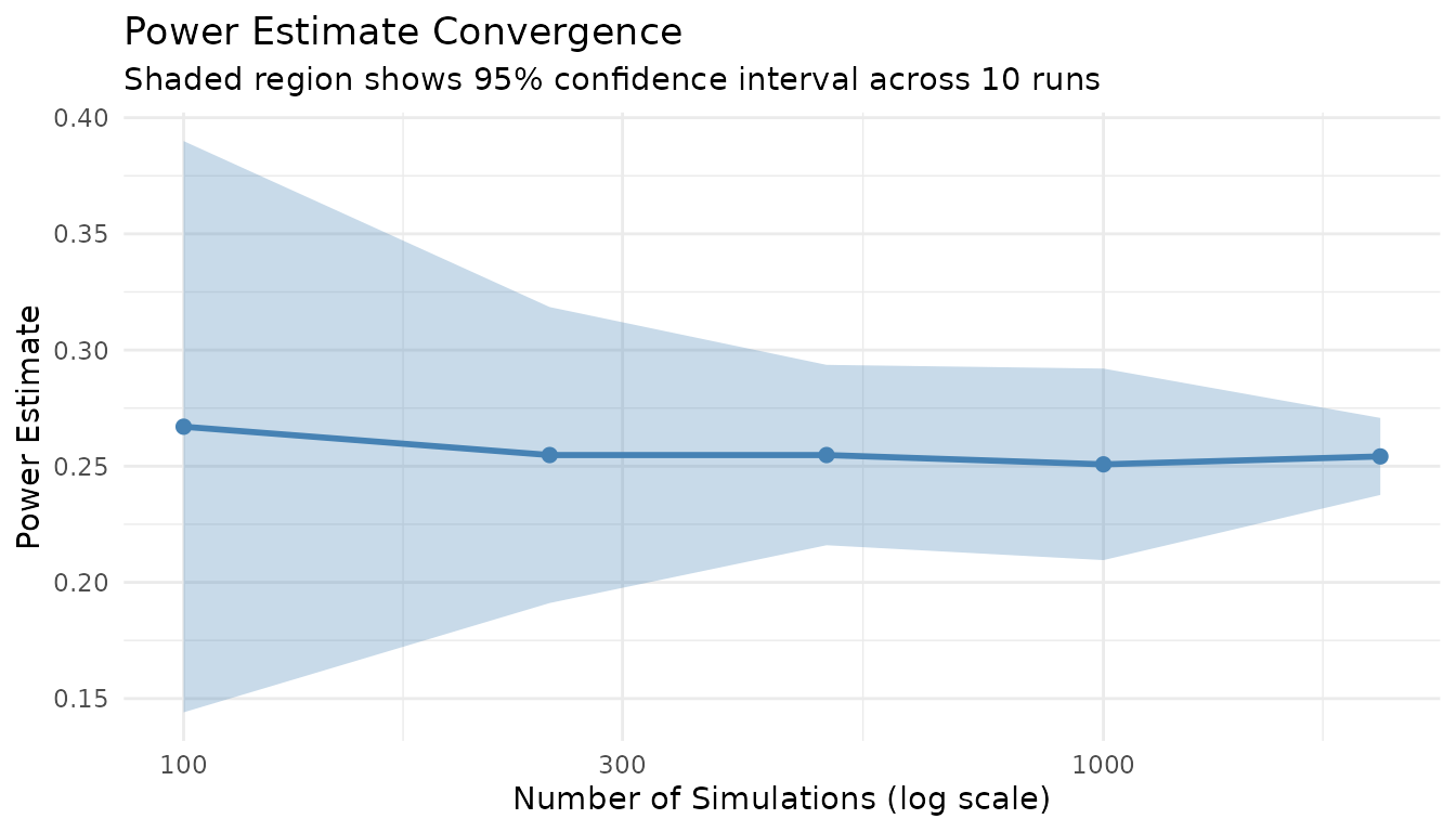
Key insight: n_sim = 1000 provides a good balance between precision (CI width ~0.03) and speed. For publication-quality results, use n_sim = 2000+.
Power Analysis - Per-Peptide Mode
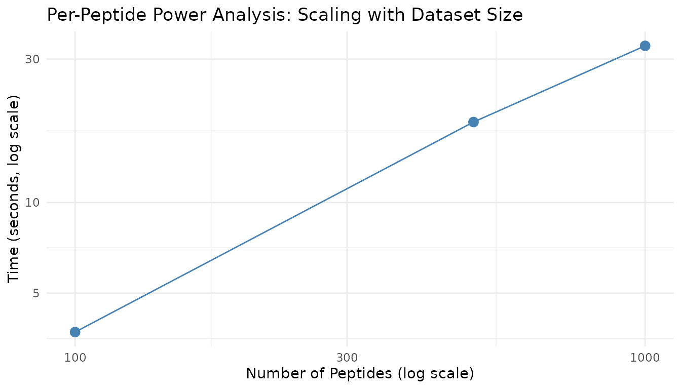
Per-peptide mode scales with both the number of peptides and n_sim.
Prepare Fits for Benchmarking
fits_100 <- fit_distributions(fit_data$n100, "peptide_id", "condition", "abundance",
                               distributions = "continuous")
fits_500 <- fit_distributions(fit_data$n500, "peptide_id", "condition", "abundance",
                               distributions = "continuous")
fits_1000 <- fit_distributions(fit_data$n1000, "peptide_id", "condition", "abundance",
                                distributions = "continuous")
Scaling by Peptide Count
set.seed(123)

pp_peptide_results <- bench::mark(
  `100 peptides` = power_analysis(fits_100, effect_size = 2, n_per_group = 6,
                                  find = "power", n_sim = 500),
  `500 peptides` = power_analysis(fits_500, effect_size = 2, n_per_group = 6,
                                  find = "power", n_sim = 500),
  `1000 peptides` = power_analysis(fits_1000, effect_size = 2, n_per_group = 6,
                                   find = "power", n_sim = 500),
  iterations = 1,
  check = FALSE
)

pp_pep_df <- tibble::tibble(
  peptides = c(100, 500, 1000),
  time_s = as.numeric(pp_peptide_results$median),
  time_per_peptide_ms = time_s * 1000 / peptides
)

knitr::kable(
  pp_pep_df,
  col.names = c("Peptides", "Time (s)", "Time/peptide (ms)"),
  digits = 2,
  caption = "Per-peptide mode scaling by peptide count (n_sim=500)"
)| Peptides | Time (s) | Time/peptide (ms) |
|---|---|---|
| 100 | 3.35 | 33.50 |
| 500 | 14.32 | 28.64 |
| 1000 | 27.12 | 27.12 |
Scaling by n_sim
set.seed(123)

pp_nsim_results <- bench::mark(
  `n_sim=250` = power_analysis(fits_500, effect_size = 2, n_per_group = 6,
                               find = "power", n_sim = 250),
  `n_sim=500` = power_analysis(fits_500, effect_size = 2, n_per_group = 6,
                               find = "power", n_sim = 500),
  `n_sim=1000` = power_analysis(fits_500, effect_size = 2, n_per_group = 6,
                                find = "power", n_sim = 1000),
  iterations = 1,
  check = FALSE
)

pp_nsim_df <- tibble::tibble(
  n_sim = c(250, 500, 1000),
  time_s = as.numeric(pp_nsim_results$median)
)

knitr::kable(
  pp_nsim_df,
  col.names = c("n_sim", "Time (s)"),
  digits = 2,
  caption = "Per-peptide mode scaling by n_sim (500 peptides)"
)| n_sim | Time (s) |
|---|---|
| 250 | 7.52 |
| 500 | 14.82 |
| 1000 | 29.24 |
Scaling Visualization
ggplot2::ggplot(pp_pep_df, ggplot2::aes(x = peptides, y = time_s)) +
  ggplot2::geom_point(size = 3, color = "steelblue") +
  ggplot2::geom_line(color = "steelblue") +
  ggplot2::scale_x_log10() +
  ggplot2::scale_y_log10() +
  ggplot2::theme_minimal() +
  ggplot2::labs(
    x = "Number of Peptides (log scale)",
    y = "Time (seconds, log scale)",
    title = "Per-Peptide Power Analysis: Scaling with Dataset Size"
  )
Recommendations
For Quick Exploratory Analysis
| Parameter | Recommendation |
|---|---|
| n_sim | 500-1000 |
| Dataset | Full or sub-sample if > 5000 peptides |
| Expected time | ~1-2 min for 1000 peptides |
For Publication-Quality Results
| Parameter | Recommendation |
|---|---|
| n_sim | 2000-5000 |
| Dataset | Full peptide set |
| Expected time | ~5-10 min for 1000 peptides |
Time Estimation Formula
For per-peptide mode:
Estimated time (s) ≈ (n_peptides × n_sim × time_per_sim) + fitting_timeWhere: - time_per_sim ≈ 0.002-0.005 seconds (depends on
test type) - fitting_time ≈ 0.02 seconds per peptide
Memory Considerations
- Fitting: ~0.1-0.2 MB per 100 peptides
- Power analysis: Minimal additional memory (results stored per peptide)
- For very large datasets (>10000 peptides), ensure at least 4GB available RAM
Statistical Test Speed Comparison
set.seed(123)

test_timing <- bench::mark(
  wilcoxon = power_analysis("gamma", list(shape = 2, rate = 0.05),
                            effect_size = 2, n_per_group = 6,
                            find = "power", test = "wilcoxon", n_sim = 500),
  bootstrap_t = power_analysis("gamma", list(shape = 2, rate = 0.05),
                               effect_size = 2, n_per_group = 6,
                               find = "power", test = "bootstrap_t", n_sim = 500),
  bayes_t = power_analysis("gamma", list(shape = 2, rate = 0.05),
                           effect_size = 2, n_per_group = 6,
                           find = "power", test = "bayes_t", n_sim = 500),
  rankprod = power_analysis("gamma", list(shape = 2, rate = 0.05),
                            effect_size = 2, n_per_group = 6,
                            find = "power", test = "rankprod", n_sim = 500),
  iterations = 2,
  check = FALSE
)

test_df <- tibble::tibble(
  test = c("wilcoxon", "bootstrap_t", "bayes_t", "rankprod"),
  time_s = as.numeric(test_timing$median),
  relative = time_s / min(time_s)
)

knitr::kable(
  test_df,
  col.names = c("Test", "Time (s)", "Relative Speed"),
  digits = 2,
  caption = "Statistical test speed comparison (n_sim=500)"
)| Test | Time (s) | Relative Speed |
|---|---|---|
| wilcoxon | 0.04 | 2.33 |
| bootstrap_t | 16.27 | 957.31 |
| bayes_t | 0.02 | 1.00 |
| rankprod | 8.41 | 495.14 |
Note: The bootstrap_t and rankprod tests are slower due to resampling procedures. For large-scale analyses, wilcoxon or bayes_t are faster options.
Missingness-Aware Simulation Performance
When include_missingness = TRUE, peppwR incorporates
peptide-specific NA rates into simulations. Let’s measure the
overhead:
# Generate data with realistic missingness
generate_test_data_with_na <- function(n_peptides, n_per_group = 4, na_rate = 0.15, seed = 42) {
  set.seed(seed)

  data <- generate_test_data(n_peptides, n_per_group, seed)

  # Introduce MNAR pattern: low values more likely to be missing
  threshold <- quantile(data$abundance, 0.3)
  data$abundance <- ifelse(
    data$abundance < threshold & runif(nrow(data)) < na_rate * 2,
    NA,
    data$abundance
  )

  # Also some random MCAR missingness
  data$abundance <- ifelse(
    runif(nrow(data)) < na_rate / 3,
    NA,
    data$abundance
  )

  data
}

data_with_na <- generate_test_data_with_na(500, n_per_group = 4, na_rate = 0.15)
fits_with_na <- fit_distributions(data_with_na, "peptide_id", "condition", "abundance",
                                   distributions = "continuous")
set.seed(123)

miss_results <- bench::mark(
  `Without missingness` = power_analysis(fits_with_na, effect_size = 2, n_per_group = 6,
                                         find = "power", n_sim = 200,
                                         include_missingness = FALSE),
  `With missingness` = power_analysis(fits_with_na, effect_size = 2, n_per_group = 6,
                                      find = "power", n_sim = 200,
                                      include_missingness = TRUE),
  iterations = 2,
  check = FALSE
)

miss_df <- tibble::tibble(
  mode = c("Without missingness", "With missingness"),
  time_s = as.numeric(miss_results$median)
)

knitr::kable(
  miss_df,
  col.names = c("Mode", "Time (s)"),
  digits = 2,
  caption = "Missingness-aware simulation overhead"
)| Mode | Time (s) |
|---|---|
| Without missingness | 4.63 |
| With missingness | 4.57 |
The overhead of include_missingness = TRUE is minimal -
it’s primarily the NA handling within the simulation loop, which is
fast.
FDR Mode Performance
FDR-aware mode simulates entire peptidome experiments with mixed null and alternative peptides, then applies BH correction. This is more computationally intensive than per-peptide mode.
set.seed(123)

fdr_results <- bench::mark(
  `Per-peptide (no FDR)` = power_analysis(fits_500, effect_size = 2, n_per_group = 6,
                                          find = "power", n_sim = 100),
  `FDR-adjusted` = power_analysis(fits_500, effect_size = 2, n_per_group = 6,
                                  find = "power", apply_fdr = TRUE,
                                  prop_null = 0.9, n_sim = 100),
  iterations = 2,
  check = FALSE
)

fdr_df <- tibble::tibble(
  mode = c("Per-peptide (no FDR)", "FDR-adjusted"),
  time_s = as.numeric(fdr_results$median)
)

knitr::kable(
  fdr_df,
  col.names = c("Mode", "Time (s)"),
  digits = 2,
  caption = "FDR mode vs per-peptide mode timing"
)| Mode | Time (s) |
|---|---|
| Per-peptide (no FDR) | 2.90 |
| FDR-adjusted | 3.42 |
FDR mode is more expensive because each simulation iteration requires: 1. Assigning peptides to null/alternative 2. Simulating all peptides together 3. Applying BH correction across all p-values
FDR Scaling with Peptide Count
set.seed(123)

fdr_scaling_results <- bench::mark(
  `100 peptides` = power_analysis(fits_100, effect_size = 2, n_per_group = 6,
                                  find = "power", apply_fdr = TRUE, n_sim = 50),
  `500 peptides` = power_analysis(fits_500, effect_size = 2, n_per_group = 6,
                                  find = "power", apply_fdr = TRUE, n_sim = 50),
  `1000 peptides` = power_analysis(fits_1000, effect_size = 2, n_per_group = 6,
                                   find = "power", apply_fdr = TRUE, n_sim = 50),
  iterations = 1,
  check = FALSE
)

fdr_scale_df <- tibble::tibble(
  peptides = c(100, 500, 1000),
  time_s = as.numeric(fdr_scaling_results$median)
)

knitr::kable(
  fdr_scale_df,
  col.names = c("Peptides", "Time (s)"),
  digits = 2,
  caption = "FDR mode scaling by peptide count (n_sim=50)"
)| Peptides | Time (s) |
|---|---|
| 100 | 0.38 |
| 500 | 1.80 |
| 1000 | 3.21 |
Diagnostic Plot Generation Times
set.seed(42)

plot_results <- bench::mark(
  `Density overlay` = plot_density_overlay(fits_500, n_overlay = 6),
  `QQ plots` = plot_qq(fits_500, n_plots = 6),
  `Param distribution` = plot_param_distribution(fits_500),
  iterations = 2,
  check = FALSE
)

plot_df <- tibble::tibble(
  plot = c("Density overlay", "QQ plots", "Param distribution"),
  time_s = as.numeric(plot_results$median)
)

knitr::kable(
  plot_df,
  col.names = c("Plot Type", "Time (s)"),
  digits = 3,
  caption = "Diagnostic plot generation times"
)| Plot Type | Time (s) |
|---|---|
| Density overlay | 0.060 |
| QQ plots | 0.037 |
| Param distribution | 0.696 |
set.seed(123)

heatmap_results <- bench::mark(
  `Power heatmap (5x5)` = plot_power_heatmap(
    "gamma", list(shape = 2, rate = 0.05),
    n_range = c(3, 12), effect_range = c(1.5, 3),
    n_steps = 5, n_sim = 50
  ),
  iterations = 1,
  check = FALSE
)

knitr::kable(
  tibble::tibble(
    plot = "Power heatmap (5x5 grid, n_sim=50)",
    time_s = as.numeric(heatmap_results$median)
  ),
  col.names = c("Plot Type", "Time (s)"),
  digits = 2,
  caption = "Power heatmap generation time"
)| Plot Type | Time (s) |
|---|---|
| Power heatmap (5x5 grid, n_sim=50) | 0.15 |
Note: The power heatmap is expensive because it runs
n_steps^2 × n_sim simulations. Use smaller grids and fewer
simulations for exploratory work.
Session Info
sessionInfo()
#> R version 4.5.3 (2026-03-11)
#> Platform: x86_64-pc-linux-gnu
#> Running under: Ubuntu 24.04.4 LTS
#>
#> Matrix products: default
#> BLAS:   /usr/lib/x86_64-linux-gnu/openblas-pthread/libblas.so.3
#> LAPACK: /usr/lib/x86_64-linux-gnu/openblas-pthread/libopenblasp-r0.3.26.so;  LAPACK version 3.12.0
#>
#> locale:
#>  [1] LC_CTYPE=C.UTF-8       LC_NUMERIC=C           LC_TIME=C.UTF-8
#>  [4] LC_COLLATE=C.UTF-8     LC_MONETARY=C.UTF-8    LC_MESSAGES=C.UTF-8
#>  [7] LC_PAPER=C.UTF-8       LC_NAME=C              LC_ADDRESS=C
#> [10] LC_TELEPHONE=C         LC_MEASUREMENT=C.UTF-8 LC_IDENTIFICATION=C
#>
#> time zone: UTC
#> tzcode source: system (glibc)
#>
#> attached base packages:
#> [1] stats     graphics  grDevices datasets  utils     methods   base
#>
#> other attached packages:
#> [1] bench_1.1.4  peppwR_0.1.0
#>
#> loaded via a namespace (and not attached):
#>  [1] sass_0.4.10         generics_0.1.4      tidyr_1.3.2
#>  [4] renv_0.12.2         fGarch_4052.93      lattice_0.22-9
#>  [7] digest_0.6.39       magrittr_2.0.5      RColorBrewer_1.1-3
#> [10] evaluate_1.0.5      grid_4.5.3          fastmap_1.2.0
#> [13] jsonlite_2.0.0      Matrix_1.7-4        purrr_1.2.2
#> [16] scales_1.4.0        gbutils_0.5.1       codetools_0.2-20
#> [19] textshaping_1.0.5   jquerylib_0.1.4     Rdpack_2.6.6
#> [22] cli_3.6.6           timeSeries_4052.112 rlang_1.2.0
#> [25] rbibutils_2.4.1     intervals_0.15.5    withr_3.0.2
#> [28] cachem_1.1.0        yaml_2.3.12         cvar_0.6
#> [31] tools_4.5.3         dplyr_1.2.1         ggplot2_4.0.2
#> [34] profmem_0.7.0       assertthat_0.2.1    vctrs_0.7.3
#> [37] R6_2.6.1            lifecycle_1.0.5     fs_2.0.1
#> [40] univariateML_1.5.0  ragg_1.5.2          pkgconfig_2.0.3
#> [43] desc_1.4.3          gtable_0.3.6        pkgdown_2.2.0
#> [46] pillar_1.11.1       bslib_0.10.0        glue_1.8.0
#> [49] systemfonts_1.3.2   xfun_0.57           tibble_3.3.1
#> [52] tidyselect_1.2.1    knitr_1.51          farver_2.1.2
#> [55] spatial_7.3-18      htmltools_0.5.9     fBasics_4052.98
#> [58] labeling_0.4.3      rmarkdown_2.31      timeDate_4052.112
#> [61] compiler_4.5.3      S7_0.2.1-1