Pan-Genome Analysis with paneffectR

Introduction

While paneffectR was designed for effector analysis, it works equally well for general pan-genome comparisons with any protein FASTA files. This vignette demonstrates how to:

Compare protein content across genome assemblies
Identify core, accessory, and unique proteins
Visualize pan-genome structure

No effector scores are required.

Pan-Genome Concepts

A pan-genome represents the complete gene content across a set of related genomes:

Core genome: Genes present in all (or nearly all) genomes - essential functions
Accessory genome: Genes present in some genomes - niche adaptation, lifestyle
Unique genes: Present in only one genome - strain-specific features

paneffectR helps you explore this structure through presence/absence analysis.

Setup

library(paneffectR)
library(dplyr)
#> 
#> Attaching package: 'dplyr'
#> The following objects are masked from 'package:stats':
#> 
#>     filter, lag
#> The following objects are masked from 'package:base':
#> 
#>     intersect, setdiff, setequal, union

Loading FASTA Files

For pan-genome analysis, you only need FASTA files:

# Get path to test data
testdata_dir <- system.file("testdata", package = "paneffectR")

# Load FASTAs only (no scores)
proteins <- load_proteins(
  fasta_dir = testdata_dir,
  pattern = "*.faa"
)
proteins
#> -- protein_collection --
#> 3 assemblies, 300 total proteins
#> 
#> # A tibble: 3 × 3
#>   assembly_name n_proteins has_scores
#>   <chr>              <int> <lgl>     
#> 1 assembly1            100 FALSE     
#> 2 assembly2            100 FALSE     
#> 3 assembly3            100 FALSE

Note: Even though our test data has scores available, we’re ignoring them for this analysis.

Protein ID Requirements

Protein IDs must be unique across all assemblies. If your FASTAs have generic headers like >protein_001, you’ll need to prefix them with assembly names.

paneffectR validates this automatically:

# This would fail if IDs weren't unique
# (our test data already has unique IDs like "assembly1_000001")
head(proteins$assemblies[[1]]$proteins$protein_id)
#> [1] "assembly1_000039" "assembly1_000040" "assembly1_000094" "assembly1_000122"
#> [5] "assembly1_000164" "assembly1_000194"

Clustering Proteins

Group proteins from different assemblies into orthogroups:

# Cluster using DIAMOND reciprocal best hits
clusters <- cluster_proteins(proteins, method = "diamond_rbh")

For this vignette, we’ll use pre-computed clusters:

visual_dir <- system.file("testdata", "visual", package = "paneffectR")
clusters <- readRDS(file.path(visual_dir, "clusters_visual.rds"))
clusters
#> -- orthogroup_result (synthetic_visual) --
#> 50 orthogroups
#> 12 singletons

Understanding the Results

# Orthogroup statistics
clusters$stats
#> # A tibble: 1 × 4
#>   n_orthogroups n_singletons n_proteins_clustered n_assemblies
#>           <int>        <int>                <int>        <int>
#> 1            50           12                  160            6

# How many singletons (unique proteins)?
n_singletons(clusters)
#> [1] 12

# Singletons per assembly
singletons_by_assembly(clusters)
#> # A tibble: 6 × 2
#>   assembly n_singletons
#>   <chr>           <int>
#> 1 asm_A               2
#> 2 asm_B               2
#> 3 asm_C               2
#> 4 asm_D               2
#> 5 asm_E               2
#> 6 asm_F               2

Building the Presence/Absence Matrix

Create a binary matrix showing which orthogroups are in which assemblies:

pa <- build_pa_matrix(clusters, type = "binary")
pa
#> -- pa_matrix (binary) --
#> 62 orthogroups x 6 assemblies
#> Sparsity: 53.8%

# Include singletons (default) or exclude them
pa_no_singletons <- build_pa_matrix(
  clusters,
  type = "binary",
  exclude_singletons = TRUE
)

cat("With singletons:", nrow(pa$matrix), "orthogroups\n")
#> With singletons: 62 orthogroups
cat("Without singletons:", nrow(pa_no_singletons$matrix), "orthogroups\n")
#> Without singletons: 50 orthogroups

Analyzing Pan-Genome Structure

Core Genome

Proteins present in all assemblies:

n_assemblies <- ncol(pa$matrix)
presence_count <- rowSums(pa$matrix)

# Core = present in all
core_og <- names(presence_count[presence_count == n_assemblies])
cat("Core orthogroups:", length(core_og), "of", length(presence_count), "\n")
#> Core orthogroups: 10 of 62
cat("Core percentage:", round(100 * length(core_og) / length(presence_count), 1), "%\n")
#> Core percentage: 16.1 %

Accessory Genome

Proteins present in some but not all assemblies:

# Accessory = present in 2 to (n-1) assemblies
accessory_og <- names(presence_count[presence_count > 1 & presence_count < n_assemblies])
cat("Accessory orthogroups:", length(accessory_og), "\n")
#> Accessory orthogroups: 30
cat("Accessory percentage:", round(100 * length(accessory_og) / length(presence_count), 1), "%\n")
#> Accessory percentage: 48.4 %

Unique Genes

Proteins present in only one assembly (including singletons):

unique_og <- names(presence_count[presence_count == 1])
cat("Unique orthogroups:", length(unique_og), "\n")
#> Unique orthogroups: 22
cat("Unique percentage:", round(100 * length(unique_og) / length(presence_count), 1), "%\n")
#> Unique percentage: 35.5 %

Pan-Genome Summary

pan_summary <- data.frame(
  Category = c("Core", "Accessory", "Unique", "Total"),
  Count = c(length(core_og), length(accessory_og), length(unique_og), length(presence_count)),
  Percentage = c(
    round(100 * length(core_og) / length(presence_count), 1),
    round(100 * length(accessory_og) / length(presence_count), 1),
    round(100 * length(unique_og) / length(presence_count), 1),
    100
  )
)
pan_summary
#>    Category Count Percentage
#> 1      Core    10       16.1
#> 2 Accessory    30       48.4
#> 3    Unique    22       35.5
#> 4     Total    62      100.0

Visualizing the Pan-Genome

Heatmap

The heatmap shows presence (colored) and absence (white) patterns:

ht <- plot_heatmap(
  pa,
  cluster_rows = TRUE,
  cluster_cols = TRUE,
  show_row_names = FALSE,
  color = c("white", "steelblue")
)
ComplexHeatmap::draw(ht)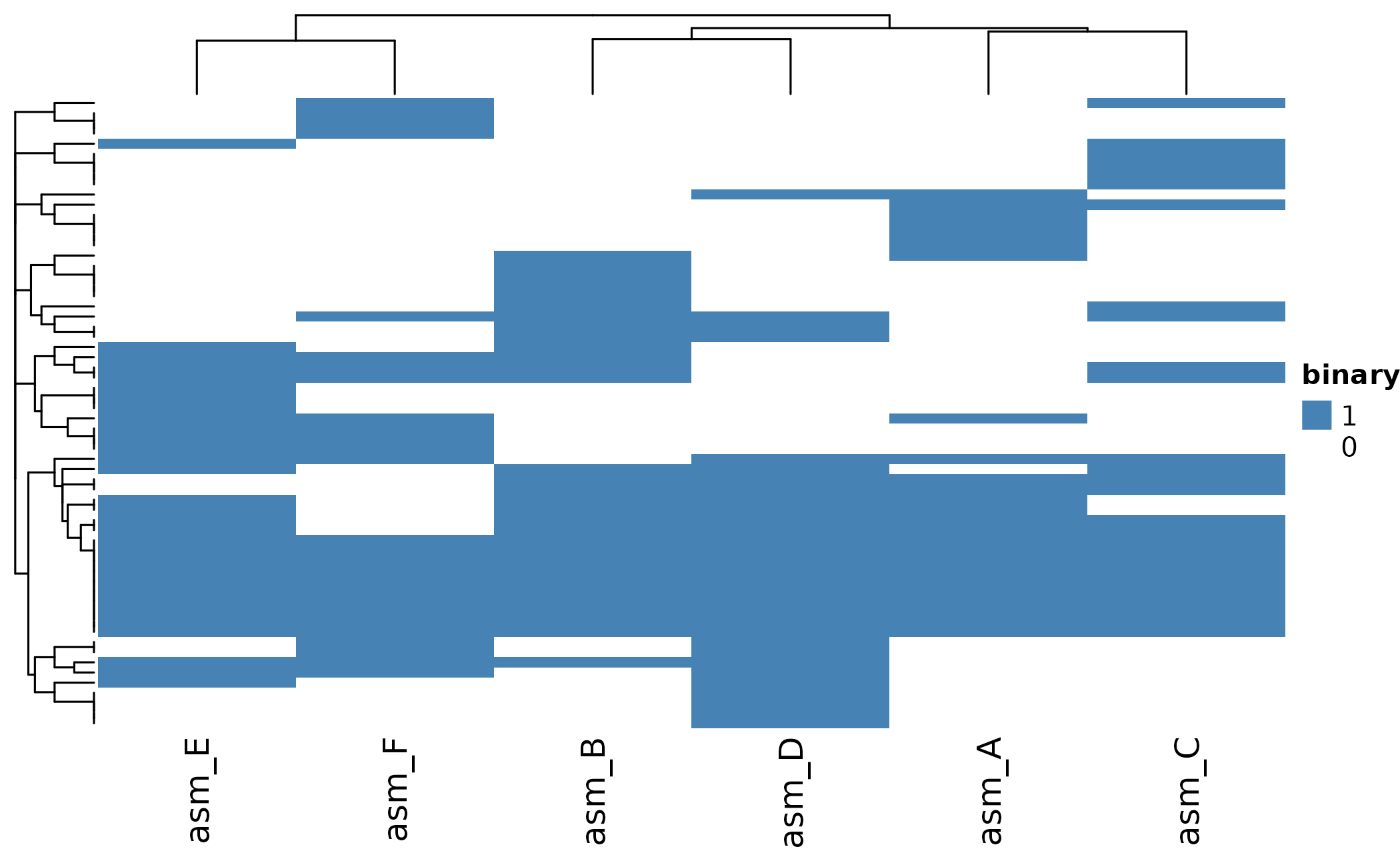

UpSet Plot

UpSet plots excel at showing intersections - which orthogroups are shared between which combinations of assemblies:

# Show all intersections with at least 1 orthogroup
plot_upset(pa, min_size = 1)
#> Warning: `aes_string()` was deprecated in ggplot2 3.0.0.
#> ℹ Please use tidy evaluation idioms with `aes()`.
#> ℹ See also `vignette("ggplot2-in-packages")` for more information.
#> ℹ The deprecated feature was likely used in the UpSetR package.
#>   Please report the issue to the authors.
#> This warning is displayed once per session.
#> Call `lifecycle::last_lifecycle_warnings()` to see where this warning was
#> generated.
#> Warning: Using `size` aesthetic for lines was deprecated in ggplot2 3.4.0.
#> ℹ Please use `linewidth` instead.
#> ℹ The deprecated feature was likely used in the UpSetR package.
#>   Please report the issue to the authors.
#> This warning is displayed once per session.
#> Call `lifecycle::last_lifecycle_warnings()` to see where this warning was
#> generated.
#> Warning: The `size` argument of `element_line()` is deprecated as of ggplot2 3.4.0.
#> ℹ Please use the `linewidth` argument instead.
#> ℹ The deprecated feature was likely used in the UpSetR package.
#>   Please report the issue to the authors.
#> This warning is displayed once per session.
#> Call `lifecycle::last_lifecycle_warnings()` to see where this warning was
#> generated.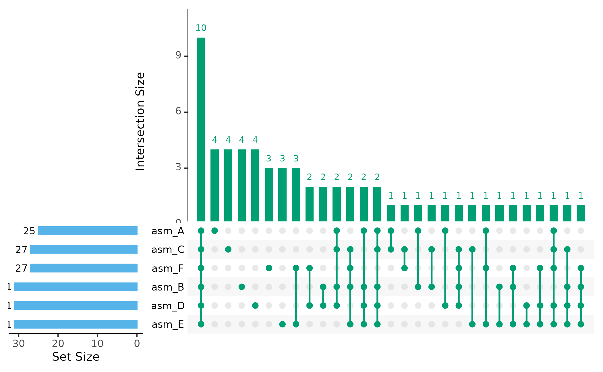

The bars show: - How many orthogroups are unique to each assembly - How many are shared between specific combinations - How many are in the core (all assemblies)

Assembly Dendrogram

Cluster assemblies by their shared protein content:

plot_dendro(pa, distance_method = "jaccard")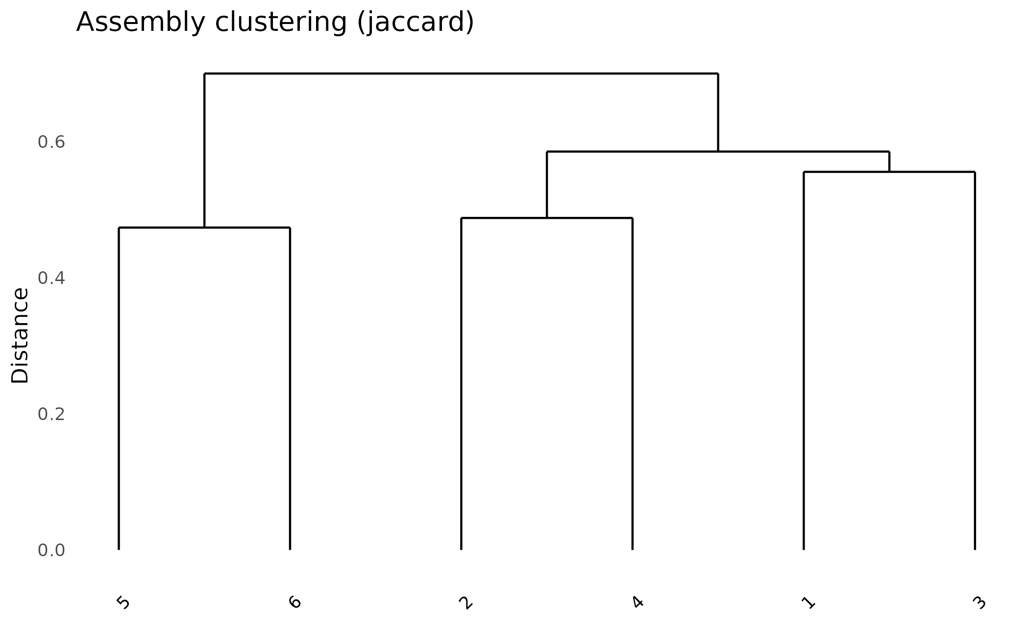

Try different distance metrics:

# Jaccard: good for presence/absence
plot_dendro(pa, distance_method = "jaccard") +
  ggplot2::ggtitle("Jaccard Distance")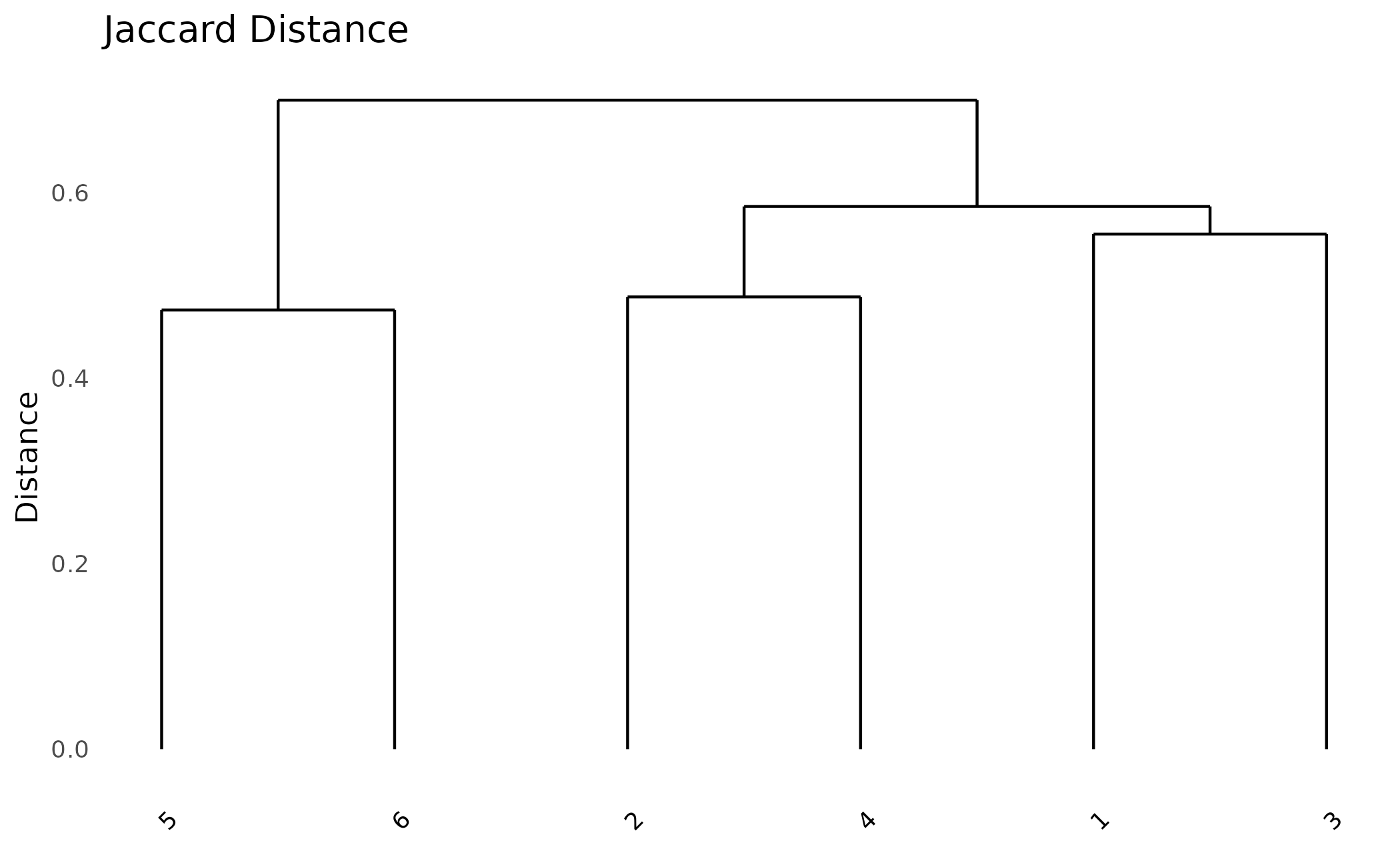

Comparing Assemblies

Pairwise Similarity

Calculate Jaccard similarity between all pairs:

# Simple Jaccard calculation
jaccard <- function(a, b) {
  intersection <- sum(a == 1 & b == 1)
  union <- sum(a == 1 | b == 1)
  intersection / union
}

# Calculate for all pairs
assemblies <- colnames(pa$matrix)
n <- length(assemblies)
sim_matrix <- matrix(0, n, n, dimnames = list(assemblies, assemblies))

for (i in 1:n) {
  for (j in 1:n) {
    sim_matrix[i, j] <- jaccard(pa$matrix[, i], pa$matrix[, j])
  }
}

round(sim_matrix, 2)
#>       asm_A asm_B asm_C asm_D asm_E asm_F
#> asm_A  1.00  0.44  0.44  0.47  0.40  0.30
#> asm_B  0.44  1.00  0.49  0.51  0.48  0.35
#> asm_C  0.44  0.49  1.00  0.41  0.41  0.38
#> asm_D  0.47  0.51  0.41  1.00  0.44  0.38
#> asm_E  0.40  0.48  0.41  0.44  1.00  0.53
#> asm_F  0.30  0.35  0.38  0.38  0.53  1.00

# Find most similar pair (excluding diagonal)
sim_matrix_upper <- sim_matrix
diag(sim_matrix_upper) <- 0
max_idx <- which(sim_matrix_upper == max(sim_matrix_upper), arr.ind = TRUE)[1, ]

cat("Most similar pair:",
    assemblies[max_idx[1]], "and", assemblies[max_idx[2]],
    "\nJaccard similarity:", round(max(sim_matrix_upper), 3), "\n")
#> Most similar pair: asm_F and asm_E 
#> Jaccard similarity: 0.526

Assembly-Specific Analysis

Proteins Unique to One Assembly

# Get singletons with assembly information
singletons_df <- singletons_by_assembly(clusters)
singletons_df
#> # A tibble: 6 × 2
#>   assembly n_singletons
#>   <chr>           <int>
#> 1 asm_A               2
#> 2 asm_B               2
#> 3 asm_C               2
#> 4 asm_D               2
#> 5 asm_E               2
#> 6 asm_F               2

# Which assembly has the most unique proteins?
singletons_df %>%
  arrange(desc(n_singletons))
#> # A tibble: 6 × 2
#>   assembly n_singletons
#>   <chr>           <int>
#> 1 asm_A               2
#> 2 asm_B               2
#> 3 asm_C               2
#> 4 asm_D               2
#> 5 asm_E               2
#> 6 asm_F               2

Orthogroups Missing from One Assembly

# Which orthogroups are missing from asm_A?
missing_from_asm_A <- pa$matrix[pa$matrix[, "asm_A"] == 0, , drop = FALSE]
cat("Orthogroups missing from asm_A:", nrow(missing_from_asm_A), "\n")
#> Orthogroups missing from asm_A: 37

Exporting Results

# Export presence/absence matrix as CSV
write.csv(
  as.data.frame(pa),
  "pan_genome_matrix.csv"
)

# Export orthogroup membership
write.csv(
  clusters$orthogroups,
  "orthogroup_membership.csv",
  row.names = FALSE
)

# Export pan-genome summary
write.csv(
  pan_summary,
  "pan_genome_summary.csv",
  row.names = FALSE
)

Summary

Key steps for pan-genome analysis:

Load FASTA files with load_proteins(fasta_dir)
Cluster into orthogroups with cluster_proteins()
Build binary matrix with build_pa_matrix(type = "binary")
Analyze core/accessory/unique proportions
Visualize with plot_heatmap(), plot_upset(), plot_dendro()

Next Steps

Getting Started - Basic workflow overview
Effector Analysis - Working with omnieff scores
Algorithm Deep Dive - Technical details on clustering