Algorithms in paneffectR • paneffectR

Introduction

This vignette walks through the DIAMOND RBH + Expansion clustering algorithm step by step, using real data from known fungal orthologs. Instead of describing algorithms conceptually, we show exactly what happens at each stage with actual sequence data.

library(paneffectR)
library(dplyr)
library(tidyr)
library(ggplot2)

The Dataset

We use 16 well-characterized proteins from three fungal species with known orthology relationships:

# Load the protein collection
clustering_dir <- system.file("testdata", "clustering", package = "paneffectR")
proteins <- readRDS(file.path(clustering_dir, "known_orthologs.rds"))

# Load expected relationships (ground truth)
expected <- read.csv(file.path(clustering_dir, "expected_orthogroups.csv"))

# Summary
proteins
#> -- protein_collection --
#> 3 assemblies, 16 total proteins
#> 
#> # A tibble: 3 × 3
#>   assembly_name n_proteins has_scores
#>   <chr>              <int> <lgl>     
#> 1 ncra                   5 FALSE     
#> 2 scer                   6 FALSE     
#> 3 spom                   5 FALSE

The dataset includes:

3 species: S. cerevisiae (budding yeast), S. pombe (fission yeast), N. crassa (bread mold)
5 conserved protein families: actin, GAPDH, histone H3, EF-1α, cytochrome c
1 species-specific singleton: mating pheromone MFA1 (only in S. cerevisiae)

expected |>
  select(protein_id, assembly, expected_og, protein_name) |>
  knitr::kable(caption = "Ground truth: expected orthogroup assignments")

Ground truth: expected orthogroup assignments
protein_id	assembly	expected_og	protein_name
scer_ACT1	scer	OG_actin	Actin
spom_act1	spom	OG_actin	Actin
ncra_act	ncra	OG_actin	Actin
scer_TDH1	scer	OG_gapdh	Glyceraldehyde-3-phosphate dehydrogenase 1
spom_tdh1	spom	OG_gapdh	Glyceraldehyde-3-phosphate dehydrogenase 1
ncra_gpd1	ncra	OG_gapdh	Glyceraldehyde-3-phosphate dehydrogenase
scer_HHT1	scer	OG_histone_h3	Histone H3
spom_hht1	spom	OG_histone_h3	Histone H3.1/H3.2
ncra_hh3	ncra	OG_histone_h3	Histone H3
scer_TEF1	scer	OG_ef1a	Elongation factor 1-alpha
spom_tef101	spom	OG_ef1a	Elongation factor 1-alpha-A
ncra_tef1	ncra	OG_ef1a	Elongation factor 1-alpha
scer_CYC1	scer	OG_cyc	Cytochrome c isoform 1
spom_cyc1	spom	OG_cyc	Cytochrome c
ncra_cyc1	ncra	OG_cyc	Cytochrome c
scer_MFA1	scer	singleton	Mating factor alpha-1

Step 1: All-vs-All Alignment

The first step runs DIAMOND blastp to compare every protein against every other protein. This produces a table of sequence similarity hits.

paneffectR runs DIAMOND with a custom output format to get the columns needed for filtering and RBH detection:

diamond blastp -d db -q proteins.faa -o hits.tsv \
  --outfmt 6 qseqid sseqid pident length qlen evalue bitscore

# Load pre-computed DIAMOND results
diamond_hits <- readRDS(file.path(clustering_dir, "diamond_hits.rds"))

# Show structure
cat("Total hits (excluding self-hits):", nrow(diamond_hits), "\n\n")
#> Total hits (excluding self-hits): 30
head(diamond_hits, 10) |>
  knitr::kable(digits = 2, caption = "DIAMOND output with computed coverage")

DIAMOND output with computed coverage
qseqid	sseqid	pident	length	qlen	bitscore	qcov
ncra_act	spom_act1	92.0	375	375	716	100.00
ncra_act	scer_ACT1	92.0	375	375	709	100.00
ncra_gpd1	spom_tdh1	69.1	333	338	463	98.52
ncra_gpd1	scer_TDH1	63.7	331	338	438	97.93
ncra_hh3	scer_HHT1	94.9	136	136	236	100.00
ncra_hh3	spom_hht1	92.6	136	136	235	100.00
ncra_tef1	spom_tef101	86.1	460	460	807	100.00
ncra_tef1	scer_TEF1	85.7	460	460	795	100.00
ncra_cyc1	spom_cyc1	70.4	108	108	175	100.00
ncra_cyc1	scer_CYC1	69.2	104	108	166	96.30

Understanding the columns

From DIAMOND directly (7 columns):

Column	Description
`qseqid`	Query protein ID
`sseqid`	Subject (hit) protein ID
`pident`	Percent sequence identity
`length`	Alignment length (amino acids)
`qlen`	Query sequence length
`evalue`	E-value (statistical significance; lower = better)
`bitscore`	Bit score (higher = better match)

Computed by paneffectR (1 column):

Column	Formula	Purpose
`qcov`	`(length / qlen) * 100`	Query coverage percentage, used for filtering

Note: This differs from the default BLAST tabular format, which includes alignment coordinates (qstart, qend, sstart, send) and gap information (mismatch, gapopen). We request only the columns needed for clustering.

Visualizing hit scores

# Get best hit between each pair
best_hits <- diamond_hits |>
  group_by(qseqid, sseqid) |>
  slice_max(bitscore, n = 1) |>
  ungroup()

# Order proteins by protein family (expected_og) to reveal ortholog blocks
protein_order <- expected |>
  arrange(expected_og, assembly) |>
  pull(protein_id)

# Convert to long format for ggplot with family-based ordering
plot_data <- best_hits |>
  mutate(
    qseqid = factor(qseqid, levels = protein_order),
    sseqid = factor(sseqid, levels = protein_order)
  )

ggplot(plot_data, aes(x = sseqid, y = qseqid, fill = bitscore)) +
  geom_tile() +
  scale_fill_viridis_c(name = "Bitscore") +

  theme_minimal() +
  theme(axis.text.x = element_text(angle = 45, hjust = 1, size = 8),
        axis.text.y = element_text(size = 8)) +
  labs(x = "Subject", y = "Query",
       title = "DIAMOND blastp hit scores (ordered by protein family)",
       subtitle = "Diagonal blocks show orthologs with high similarity")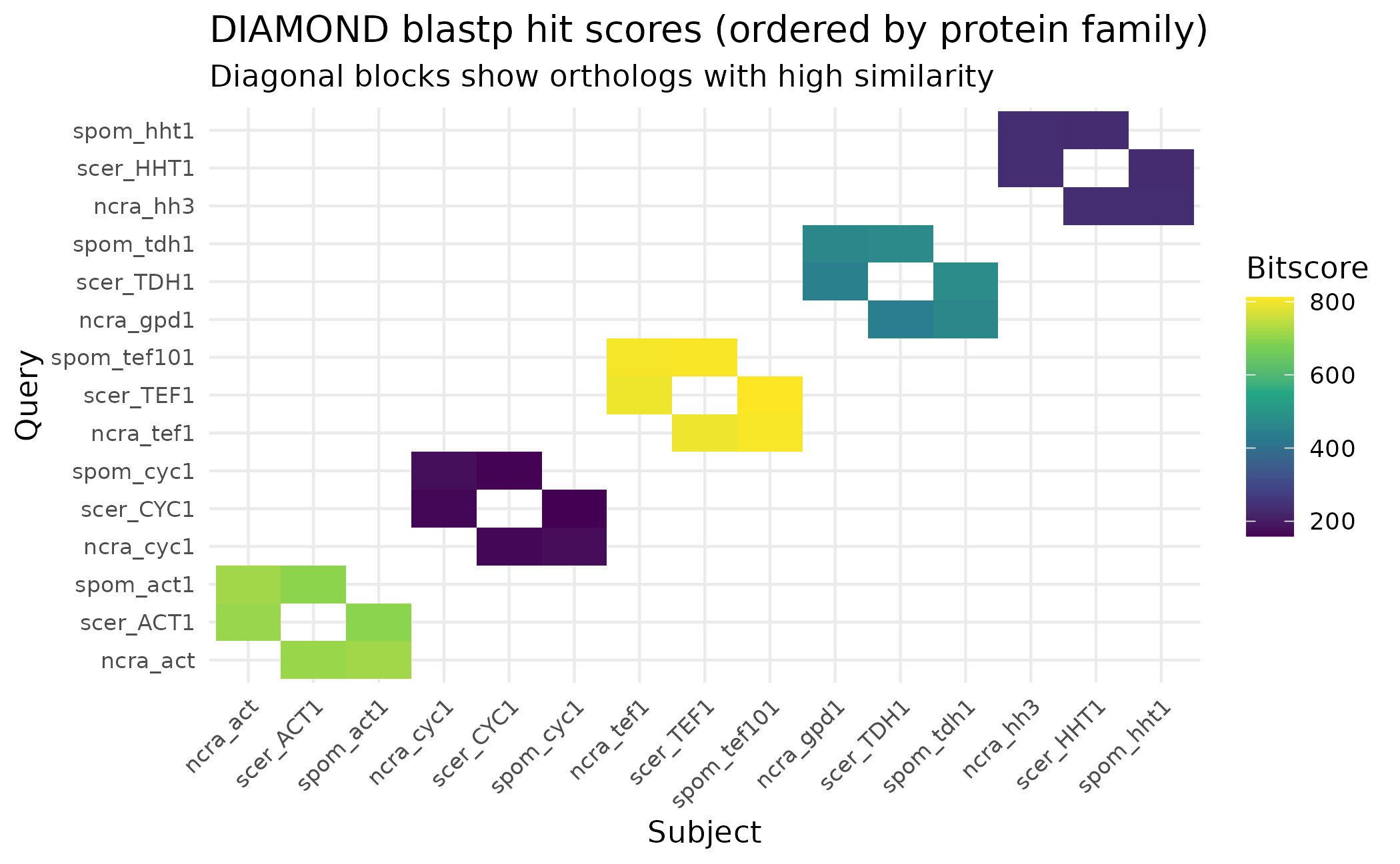

The heatmap reveals clear ortholog groups: proteins from the same family (e.g., all three actins) cluster together with high scores, while unrelated proteins show no hits.

Note: The singleton scer_MFA1 (mating pheromone) is absent from this plot because it has no significant hits to any other protein - exactly why it will end up as a singleton in the final clustering.

Step 2: Filtering by Thresholds

Not all hits are meaningful. We apply thresholds to keep only significant matches:

Parameter	Default	Purpose
`min_identity`	30%	Exclude very divergent matches
`min_coverage`	50%	Exclude partial matches
`evalue`	1e-5	Exclude statistically insignificant matches

# Load filtered hits
hits_filtered <- readRDS(file.path(clustering_dir, "diamond_hits_filtered.rds"))

cat("Before filtering:", nrow(diamond_hits), "hits\n")
#> Before filtering: 30 hits
cat("After filtering: ", nrow(hits_filtered), "hits\n")
#> After filtering:  30 hits

In this case, all hits pass the filters because these are well-conserved proteins with high sequence similarity.

Step 3: Finding Reciprocal Best Hits

A reciprocal best hit (RBH) is when two proteins are each other’s best match. This is a stringent criterion for orthology:

Find protein A’s best hit → B
Find protein B’s best hit → back to A?
If yes, A and B are reciprocal best hits

From our 30 filtered hits, paneffectR identified 5 RBH pairs:

rbh_pairs <- readRDS(file.path(clustering_dir, "rbh_pairs.rds"))

rbh_pairs |>
  knitr::kable(caption = "Reciprocal best hit pairs identified")

Reciprocal best hit pairs identified
protein_a	protein_b
ncra_act	spom_act1
ncra_cyc1	spom_cyc1
ncra_hh3	scer_HHT1
scer_TDH1	spom_tdh1
scer_TEF1	spom_tef101

Why not all orthologs form RBH pairs

Let’s trace through an example where RBH fails to connect obvious orthologs.

Question: Is scer_ACT1 (yeast actin) in an RBH pair with ncra_act (N. crassa actin)?

Step 1: Find scer_ACT1’s best hit.

scer_act1_hits <- hits_filtered |>
  filter(qseqid == "scer_ACT1") |>
  arrange(desc(bitscore))

scer_act1_hits |>
  select(qseqid, sseqid, pident, bitscore) |>
  knitr::kable()

qseqid	sseqid	pident	bitscore
scer_ACT1	ncra_act	92.0	708
scer_ACT1	spom_act1	89.6	696

The best hit (highest bitscore) is ncra_act with score 708.

Step 2: Check the reverse - what is ncra_act’s best hit?

ncra_act_hits <- hits_filtered |>
  filter(qseqid == "ncra_act") |>
  arrange(desc(bitscore))

ncra_act_hits |>
  select(qseqid, sseqid, pident, bitscore) |>
  knitr::kable()

qseqid	sseqid	pident	bitscore
ncra_act	spom_act1	92	716
ncra_act	scer_ACT1	92	709

The best hit for ncra_act is spom_act1 (score 716), not scer_ACT1 (score 709).

Result: scer_ACT1 → ncra_act, but ncra_act → spom_act1. The relationship is not reciprocal, so they are not an RBH pair.

This illustrates the limitation of pure RBH: scer_ACT1 is a clear actin ortholog, but because ncra_act is slightly more similar to spom_act1, the yeast actin gets left out of the RBH network. The expansion phase (Step 5) will rescue it.

Visualizing RBH pairs

With only 5 RBH pairs from 15 orthologous proteins, we’re clearly missing connections. To see the pattern, let’s visualize which species are linked by RBH for each protein family.

The figure below shows all 5 RBH pairs as lines connecting proteins across species. Each column is a protein family, each row is a species. Notice that RBH pairs only connect two species at a time - this is the fundamental limitation that the expansion phase addresses.

# Get protein positions for network layout
protein_positions <- expected |>
  filter(expected_og != "singleton") |>
  mutate(
    x = as.numeric(factor(expected_og)),
    y = as.numeric(factor(assembly, levels = c("ncra", "spom", "scer")))
  )

# Plot
ggplot() +
  # Add edges for RBH pairs
  geom_segment(
    data = rbh_pairs |>
      left_join(protein_positions |> select(protein_id, x, y),
                by = c("protein_a" = "protein_id")) |>
      rename(x1 = x, y1 = y) |>
      left_join(protein_positions |> select(protein_id, x, y),
                by = c("protein_b" = "protein_id")) |>
      rename(x2 = x, y2 = y),
    aes(x = x1, y = y1, xend = x2, yend = y2),
    color = "steelblue", linewidth = 1.5, alpha = 0.6
  ) +
  # Add protein points
  geom_point(data = protein_positions,
             aes(x = x, y = y, color = assembly),
             size = 4) +
  geom_text(data = protein_positions,
            aes(x = x, y = y, label = protein_id),
            size = 2.5, vjust = -1) +
  scale_y_continuous(
    breaks = 1:3,
    labels = c("N. crassa", "S. pombe", "S. cerevisiae")
  ) +
  scale_x_continuous(
    breaks = 1:5,
    labels = c("actin", "cyc", "ef1a", "gapdh", "h3")
  ) +
  scale_color_manual(values = c(ncra = "#E69F00", spom = "#56B4E9", scer = "#009E73")) +
  theme_minimal() +
  labs(title = "RBH pairs connect proteins across species",
       subtitle = "Lines show reciprocal best hit relationships",
       x = "Protein family", y = NULL) +
  theme(legend.position = "none",
        panel.grid.minor = element_blank())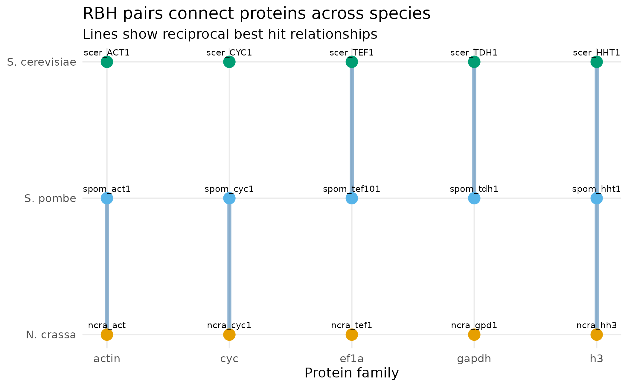

Notice that RBH pairs only connect two species at a time. This is the fundamental limitation of pure RBH: it can’t directly identify orthogroups spanning three or more species.

Step 4: Building Seed Clusters

The RBH pairs form the “seeds” for orthogroups. We find connected components in the RBH graph: proteins linked through any chain of RBH pairs form one group.

orthogroups_seed <- readRDS(file.path(clustering_dir, "orthogroups_seed.rds"))

orthogroups_seed |>
  arrange(orthogroup_id, protein_id) |>
  knitr::kable(caption = "Seed orthogroups from RBH connected components")

Seed orthogroups from RBH connected components
orthogroup_id	protein_id
OG0001	ncra_act
OG0001	spom_act1
OG0002	ncra_cyc1
OG0002	spom_cyc1
OG0003	ncra_hh3
OG0003	scer_HHT1
OG0004	scer_TDH1
OG0004	spom_tdh1
OG0005	scer_TEF1
OG0005	spom_tef101

After the seed phase:

5 orthogroups with 10 proteins (2 proteins each)
6 singletons: proteins not in any RBH pair

seed_summary <- orthogroups_seed |>
  group_by(orthogroup_id) |>
  summarize(n_proteins = n(), proteins = paste(protein_id, collapse = ", "))

seed_summary |>
  knitr::kable(caption = "Seed orthogroup composition")

Seed orthogroup composition
orthogroup_id	n_proteins	proteins
OG0001	2	ncra_act, spom_act1
OG0002	2	ncra_cyc1, spom_cyc1
OG0003	2	ncra_hh3, scer_HHT1
OG0004	2	scer_TDH1, spom_tdh1
OG0005	2	scer_TEF1, spom_tef101


# List singletons
all_proteins_list <- unlist(lapply(proteins$assemblies, function(ps) ps$proteins$protein_id))
singletons <- setdiff(all_proteins_list, orthogroups_seed$protein_id)
cat("\nSingletons after seed phase:", paste(singletons, collapse = ", "), "\n")
#> 
#> Singletons after seed phase: ncra_gpd1, ncra_tef1, scer_ACT1, scer_CYC1, scer_MFA1, spom_hht1

The actins (scer_ACT1), GAPDH (ncra_gpd1), cytochrome c (scer_CYC1), EF-1α (ncra_tef1), and histone H3 (spom_hht1) are all singletons - they weren’t part of any RBH pair even though they have clear orthologs!

Step 5: Expansion Phase

The expansion phase addresses the RBH limitation by adding singletons to existing orthogroups when their best hit is already a cluster member:

For each singleton, find its best hit
If that hit is in an orthogroup, add the singleton to that group
Repeat until no more proteins can be added

The DIAMOND hits behind RBH pairs

First, let’s see the actual DIAMOND output rows that support the 5 RBH pairs. For each RBH pair, both directions must be best hits:

# Get the DIAMOND hits that form RBH pairs
# For each RBH pair, show both directions from the original DIAMOND output
rbh_evidence <- rbh_pairs |>
  rowwise() |>
  mutate(
    # Get hit A -> B
    hit_ab = list(hits_filtered |>
      filter(qseqid == protein_a, sseqid == protein_b) |>
      select(qseqid, sseqid, pident, bitscore)),
    # Get hit B -> A
    hit_ba = list(hits_filtered |>
      filter(qseqid == protein_b, sseqid == protein_a) |>
      select(qseqid, sseqid, pident, bitscore))
  ) |>
  ungroup()

# Combine into one table
rbh_hits <- bind_rows(
  bind_rows(rbh_evidence$hit_ab),
  bind_rows(rbh_evidence$hit_ba)
) |>
  arrange(qseqid, desc(bitscore))

rbh_hits |>
  knitr::kable(
    caption = "DIAMOND hits for RBH pairs (both directions)",
    col.names = c("Query", "Subject", "% Identity", "Bitscore"),
    digits = 1
  )

DIAMOND hits for RBH pairs (both directions)
Query	Subject	% Identity	Bitscore
ncra_act	spom_act1	92.0	716
ncra_cyc1	spom_cyc1	70.4	175
ncra_hh3	scer_HHT1	94.9	236
scer_HHT1	ncra_hh3	94.9	235
scer_TDH1	spom_tdh1	70.7	475
scer_TEF1	spom_tef101	87.1	812
spom_act1	ncra_act	92.0	716
spom_cyc1	ncra_cyc1	70.4	177
spom_tdh1	scer_TDH1	70.7	470
spom_tef101	scer_TEF1	86.7	808

Each protein in an RBH pair has the other as its top hit (highest bitscore).

The DIAMOND hits behind expansion

Now let’s see the DIAMOND evidence for expansion. Each singleton’s best hit must be in an existing cluster:

expansion_trace <- readRDS(file.path(clustering_dir, "expansion_trace.rds"))

# For each singleton, show its DIAMOND hits (best hit first)
singletons_list <- expansion_trace$singleton

singleton_hits <- hits_filtered |>
  filter(qseqid %in% singletons_list) |>
  group_by(qseqid) |>
  arrange(desc(bitscore)) |>
  slice_head(n = 2) |>  # Show top 2 hits for context
  ungroup() |>
  select(qseqid, sseqid, pident, bitscore)

# Add cluster membership info
clustered_proteins <- orthogroups_seed$protein_id
singleton_hits <- singleton_hits |>
  mutate(
    hit_in_cluster = ifelse(sseqid %in% clustered_proteins, "Yes", "No")
  )

singleton_hits |>
  knitr::kable(
    caption = "DIAMOND hits from singletons (top 2 per singleton)",
    col.names = c("Singleton", "Hit", "% Identity", "Bitscore", "Hit in cluster?"),
    digits = 1
  )

DIAMOND hits from singletons (top 2 per singleton)
Singleton	Hit	% Identity	Bitscore	Hit in cluster?
ncra_gpd1	spom_tdh1	69.1	463	Yes
ncra_gpd1	scer_TDH1	63.7	438	Yes
ncra_tef1	spom_tef101	86.1	807	Yes
ncra_tef1	scer_TEF1	85.7	795	Yes
scer_ACT1	ncra_act	92.0	708	Yes
scer_ACT1	spom_act1	89.6	696	Yes
scer_CYC1	ncra_cyc1	69.2	165	Yes
scer_CYC1	spom_cyc1	70.2	159	Yes
spom_hht1	ncra_hh3	92.6	235	Yes
spom_hht1	scer_HHT1	92.6	232	Yes

For each singleton, the best hit (highest bitscore) is already in a seed cluster, so the singleton joins that cluster.

# Summarize the joins
expansion_trace |>
  select(singleton, best_hit, best_hit_bitscore, target_cluster) |>
  knitr::kable(
    caption = "Expansion decisions: singleton joins cluster via best hit",
    col.names = c("Singleton", "Best hit", "Bitscore", "Joins cluster"),
    digits = 0
  )

Expansion decisions: singleton joins cluster via best hit
Singleton	Best hit	Bitscore	Joins cluster
ncra_gpd1	spom_tdh1	463	OG0004
ncra_tef1	spom_tef101	807	OG0005
scer_ACT1	ncra_act	708	OG0001
scer_CYC1	ncra_cyc1	165	OG0002
spom_hht1	ncra_hh3	235	OG0003

Visualizing the clustering network

The network below shows how DIAMOND scores connect proteins. Edge thickness and labels show bitscores from the DIAMOND output. Blue edges are RBH pairs (seeds); orange edges show expansion connections.

library(igraph)

# Build edges from RBH pairs with their DIAMOND scores
rbh_with_scores <- rbh_pairs |>
  left_join(
    hits_filtered |> select(qseqid, sseqid, bitscore),
    by = c("protein_a" = "qseqid", "protein_b" = "sseqid")
  ) |>
  left_join(
    hits_filtered |> select(qseqid, sseqid, bitscore),
    by = c("protein_a" = "sseqid", "protein_b" = "qseqid"),
    suffix = c("", "_rev")
  ) |>
  mutate(bitscore = coalesce(bitscore, bitscore_rev)) |>
  select(from = protein_a, to = protein_b, bitscore) |>
  mutate(type = "RBH (seed)")

# Expansion edges already have scores
expansion_with_scores <- expansion_trace |>
  select(from = singleton, to = best_hit, bitscore = best_hit_bitscore) |>
  mutate(type = "Expansion")

# Combine all edges
all_edges <- bind_rows(rbh_with_scores, expansion_with_scores)

# Get node info (exclude singleton MFA1 which has no edges)
nodes <- expected |>
  filter(expected_og != "singleton") |>
  select(protein_id, assembly, expected_og)

# Create igraph object
g <- graph_from_data_frame(all_edges, directed = FALSE, vertices = nodes)

# Use Fruchterman-Reingold layout for natural clustering
set.seed(42)
layout <- layout_with_fr(g)
# Scale up to increase distance between nodes
layout <- layout * 2
layout_df <- as.data.frame(layout)
names(layout_df) <- c("x", "y")
layout_df$protein_id <- V(g)$name

# Add node attributes
layout_df <- layout_df |>
  left_join(nodes, by = "protein_id")

# Prepare edge coordinates
edge_df <- all_edges |>
  left_join(layout_df |> select(protein_id, x, y), by = c("from" = "protein_id")) |>
  rename(x1 = x, y1 = y) |>
  left_join(layout_df |> select(protein_id, x, y), by = c("to" = "protein_id")) |>
  rename(x2 = x, y2 = y) |>
  mutate(
    xmid = (x1 + x2) / 2,
    ymid = (y1 + y2) / 2,
    score_label = round(bitscore)
  )

# Plot
ggplot() +
  # RBH edges (solid, fixed width)
  geom_segment(
    data = filter(edge_df, type == "RBH (seed)"),
    aes(x = x1, y = y1, xend = x2, yend = y2),
    color = "steelblue", linewidth = 1.5, alpha = 0.8
  ) +
  # Expansion edges (dashed, fixed width)
  geom_segment(
    data = filter(edge_df, type == "Expansion"),
    aes(x = x1, y = y1, xend = x2, yend = y2),
    color = "darkorange", linewidth = 1.5, linetype = "dashed", alpha = 0.8
  ) +
  # Protein nodes (large)
  geom_point(
    data = layout_df,
    aes(x = x, y = y, color = assembly),
    size = 14
  ) +
  # Protein labels (inside nodes)
  geom_text(
    data = layout_df,
    aes(x = x, y = y, label = protein_id),
    size = 4.4, fontface = "bold", color = "black"
  ) +
  # Edge score labels
  geom_text(
    data = edge_df,
    aes(x = xmid, y = ymid, label = score_label),
    size = 6, fontface = "bold"
  ) +
  scale_color_manual(
    values = c(ncra = "#E69F00", spom = "#56B4E9", scer = "#009E73"),
    labels = c(ncra = "N. crassa", spom = "S. pombe", scer = "S. cerevisiae")
  ) +
  coord_cartesian(clip = "off") +
  expand_limits(x = c(min(layout_df$x) - 0.5, max(layout_df$x) + 0.5),
                y = c(min(layout_df$y) - 0.5, max(layout_df$y) + 0.5)) +
  theme_void() +
  labs(
    title = "Clustering network with DIAMOND bitscores",
    subtitle = "Blue solid = RBH pairs (seed clusters), Orange dashed = expansion joins",
    color = "Species"
  ) +
  theme(
    legend.position = "bottom",
    plot.title = element_text(hjust = 0.5, face = "bold"),
    plot.subtitle = element_text(hjust = 0.5)
  )

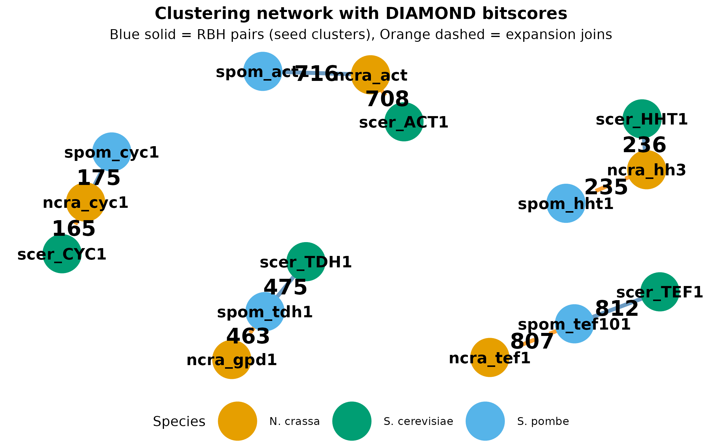
The network naturally clusters into 5 groups (the orthogroups). Proteins with high DIAMOND scores are pulled together. Notice how each orthogroup has 3 members connected by a mix of RBH (seed) and expansion edges.

What happened in expansion

Take scer_ACT1 as an example:

It’s not in an RBH pair (its best hit ncra_act prefers spom_act1)
But ncra_act IS in OG0001 (via RBH with spom_act1)
So scer_ACT1 joins OG0001 through its best-hit connection

This “anchor and expand” strategy lets orthogroups grow beyond strict RBH pairs while maintaining the high-confidence RBH relationships as a foundation.

In iteration 1, all 5 “missing” orthologs found their way home:

# Show before and after with expected orthogroup names
orthogroups_expanded <- readRDS(file.path(clustering_dir, "orthogroups_expanded.rds"))

# Add expected orthogroup info
protein_info <- expected |>
  select(protein_id, expected_og)

cat("=== Before Expansion (Seed Phase) ===\n")
#> === Before Expansion (Seed Phase) ===
orthogroups_seed |>
  left_join(protein_info, by = "protein_id") |>
  group_by(orthogroup_id) |>
  summarize(
    protein_family = first(expected_og),
    members = paste(sort(protein_id), collapse = ", ")
  ) |>
  knitr::kable()

orthogroup_id	protein_family	members
OG0001	OG_actin	ncra_act, spom_act1
OG0002	OG_cyc	ncra_cyc1, spom_cyc1
OG0003	OG_histone_h3	ncra_hh3, scer_HHT1
OG0004	OG_gapdh	scer_TDH1, spom_tdh1
OG0005	OG_ef1a	scer_TEF1, spom_tef101


cat("\n=== After Expansion ===\n")
#> 
#> === After Expansion ===
orthogroups_expanded |>
  left_join(protein_info, by = "protein_id") |>
  group_by(orthogroup_id) |>
  summarize(
    protein_family = first(expected_og),
    members = paste(sort(protein_id), collapse = ", "),
    n = n()
  ) |>
  knitr::kable()

orthogroup_id	protein_family	members	n
OG0001	OG_actin	ncra_act, scer_ACT1, spom_act1	3
OG0002	OG_cyc	ncra_cyc1, scer_CYC1, spom_cyc1	3
OG0003	OG_histone_h3	ncra_hh3, scer_HHT1, spom_hht1	3
OG0004	OG_gapdh	ncra_gpd1, scer_TDH1, spom_tdh1	3
OG0005	OG_ef1a	ncra_tef1, scer_TEF1, spom_tef101	3


# Check singleton
final_singletons <- setdiff(all_proteins_list, orthogroups_expanded$protein_id)
cat("\nFinal singleton:", final_singletons, "\n")
#> 
#> Final singleton: scer_MFA1

All 5 protein families now have their complete set of 3 orthologs, and scer_MFA1 correctly remains a singleton.

Effect of Parameters

What happens with stricter thresholds? Let’s compare:

# Load strict parameter results
hits_strict <- readRDS(file.path(clustering_dir, "diamond_hits_strict.rds"))
orthogroups_strict <- readRDS(file.path(clustering_dir, "orthogroups_strict.rds"))

cat("Default parameters (min_identity = 30%):\n")
#> Default parameters (min_identity = 30%):
cat("  Hits passing filter:", nrow(hits_filtered), "\n")
#>   Hits passing filter: 30
cat("  Orthogroups:", length(unique(orthogroups_expanded$orthogroup_id)), "\n")
#>   Orthogroups: 5
cat("  Proteins in orthogroups:", nrow(orthogroups_expanded), "\n")
#>   Proteins in orthogroups: 15

cat("\nStrict parameters (min_identity = 70%):\n")
#> 
#> Strict parameters (min_identity = 70%):
cat("  Hits passing filter:", nrow(hits_strict), "\n")
#>   Hits passing filter: 24
cat("  Orthogroups:", length(unique(orthogroups_strict$orthogroup_id)), "\n")
#>   Orthogroups: 5
cat("  Proteins in orthogroups:", nrow(orthogroups_strict), "\n")
#>   Proteins in orthogroups: 14

Which proteins are affected?

# Find proteins that got excluded
proteins_strict <- orthogroups_strict$protein_id
proteins_default <- orthogroups_expanded$protein_id

newly_singletons <- setdiff(proteins_default, proteins_strict)

cat("Proteins excluded by strict parameters:\n")
#> Proteins excluded by strict parameters:
expected |>
  filter(protein_id %in% newly_singletons) |>
  select(protein_id, protein_name, expected_og) |>
  knitr::kable()

protein_id	protein_name	expected_og
ncra_gpd1	Glyceraldehyde-3-phosphate dehydrogenase	OG_gapdh


# Show the excluded hits
hits_filtered |>
  filter(!qseqid %in% proteins_strict | !sseqid %in% proteins_strict) |>
  filter(qseqid %in% newly_singletons | sseqid %in% newly_singletons) |>
  select(qseqid, sseqid, pident, bitscore) |>
  distinct() |>
  knitr::kable(caption = "Hits excluded by 70% identity threshold")

Hits excluded by 70% identity threshold
qseqid	sseqid	pident	bitscore
ncra_gpd1	spom_tdh1	69.1	463
ncra_gpd1	scer_TDH1	63.7	438
scer_TDH1	ncra_gpd1	63.7	441
spom_tdh1	ncra_gpd1	69.1	461

The GAPDH and cytochrome c families have cross-species identities around 63-69%, below the strict 70% threshold. These proteins become incorrectly isolated as singletons with overly strict parameters.

Distance Metrics

Once orthogroups are assigned, we can build a presence/absence matrix (rows = orthogroups, columns = assemblies). To compare how similar two assemblies are based on their shared orthogroup content, we need a distance metric. This is used for hierarchical clustering and visualizations like dendrograms.

Jaccard Distance (Recommended)

The Jaccard index measures similarity as the size of the intersection divided by the size of the union. The distance is 1 minus this similarity, ignoring shared absences: $d_{Jaccard}(A, B) = 1 - \frac{|A \cap B|}{|A \cup B|}$

# Load example data from visual testdata
visual_dir <- system.file("testdata", "visual", package = "paneffectR")
pa <- readRDS(file.path(visual_dir, "pa_binary.rds"))

plot_dendro(pa, distance_method = "jaccard") +
  ggtitle("Assembly clustering with Jaccard distance")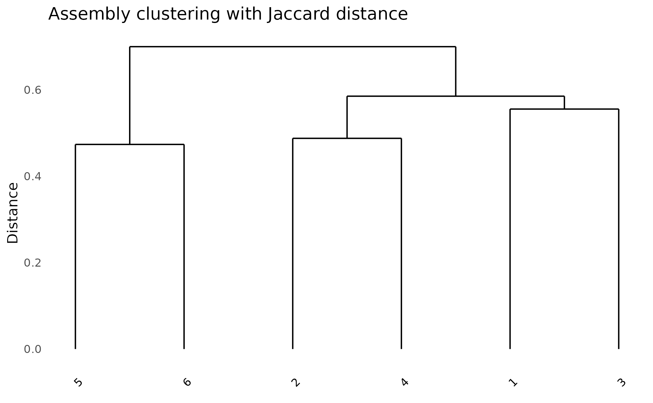

Other distance options

Binary (Euclidean): Square root of the number of orthogroups where two assemblies differ.

Bray-Curtis: Originally designed for abundance data, but works with binary. See Wikipedia.

Method	Best for
`jaccard`	Presence/absence data (default)
`binary`	When total differences matter more than proportions
`bray`	Abundance or score data

Hierarchical Clustering Methods

After computing distances, assemblies are clustered hierarchically:

Method	Behavior
`complete`	Conservative - maximizes distances between clusters
`average`	Balanced - common in phylogenetics
`ward.D2`	Creates distinct, equal-sized clusters

# Compare methods
plot_dendro(pa, cluster_method = "complete")
plot_dendro(pa, cluster_method = "average")
plot_dendro(pa, cluster_method = "ward.D2")

Handling Singletons

Singletons are proteins not assigned to any orthogroup. They may represent:

True unique genes: Horizontally transferred, species-specific
Divergent homologs: Too different to pass similarity thresholds
Artifacts: Mis-predicted ORFs, fragmented assemblies

# Using the visual test data
visual_dir <- system.file("testdata", "visual", package = "paneffectR")
clusters <- readRDS(file.path(visual_dir, "clusters_visual.rds"))

# Compare with and without singletons
pa_with <- build_pa_matrix(clusters, exclude_singletons = FALSE)
pa_without <- build_pa_matrix(clusters, exclude_singletons = TRUE)

cat("With singletons:", nrow(pa_with$matrix), "orthogroups\n")
#> With singletons: 62 orthogroups
cat("Without singletons:", nrow(pa_without$matrix), "orthogroups\n")
#> Without singletons: 50 orthogroups

When to include singletons: - Analyzing unique gene content - Calculating pan-genome size - Studying accessory genome

When to exclude singletons: - Focusing on shared variation - Phylogenetic analysis - Reducing noise

Future Additions

The cluster_proteins() function is designed to support multiple clustering backends. Currently only DIAMOND RBH is implemented, but the interface accepts a method parameter for future expansion:

cluster_proteins(proteins, method = "diamond_rbh")  # Current default
cluster_proteins(proteins, method = "orthofinder")  # Planned
cluster_proteins(proteins, method = "mmseqs2")      # Planned

OrthoFinder

OrthoFinder infers orthogroups using gene trees and is considered a gold standard for orthology inference. It handles paralogs more rigorously than RBH-based methods but requires more computation time.

MMseqs2

MMseqs2 provides ultra-fast protein clustering suitable for very large datasets. Its greedy clustering approach trades some sensitivity for speed, making it useful when analysing hundreds of assemblies.